
4-bit LLM training and Primer on Precision, data types & Quantization
Ever wondered how/why to train model in low precision? What is fp32, bfloat16? Need for quantization? Role in training/inference & tuning? Look no further, this article covers all of this and more.

TABLE OF CONTENT
Introduction: The Precision Problem in Training LLMs
Primer on Precision in Machine Learning: The Importance of Data Types
Why Should We Care About Precision?
What is Model Precision?
Comparing Precision to Image Resolution
Floating-Point Representation: Mantissa, Exponent, and Sign Bit
common data types/representations
Few fundamental questions and their plausible answers
But, how does bit reduction help? Why only reduction in mantissa?
But, why do lower precision helps in speed up?
But, why does the error accumulation happens?
How is quantization generally performed?
How Engineers Handle Precision to Scale LLMs
During Training: Mixed Precision Training
Post-Training: Post-Training Quantization (PTQ)
Optimization during Fine-Tuning: Techniques like QLoRA
Inference: Ultra-Low Precision (INT4 and Beyond)
Ideal situation, problems associated and proposed solution for 4-bit training
Methodology
Forward pass
Backward pass
How to handle and quantize activations
How to handle de-quantization using DEGs (for smoother grad updates)
Results/outcomes
Thoughts
Conclusion
Introduction: The Precision Problem in Training LLMs
Training large language models (LLMs) is one of the most computationally expensive and complex tasks in modern AI. These models, often containing billions of parameters, require not just vast amounts of data but also immense computational power. As models scale up, so do the time, cost, and resources required to train them. One of the core issues in scaling LLMs is the challenge of precision, specifically related to floating-point operations. Every single operation in training these models—be it weight updates, backpropagation, or gradient calculations—relies on floating-point arithmetic.
However, using high-precision floating-point formats (such as FP32, or 32-bit floating-point) can be prohibitively slow. This high precision is needed for accuracy, but it comes at the cost of memory and computational efficiency. For context, consider training a model like GPT-3, which requires massive computational resources. If every operation is computed in FP32, we are talking about an exponential increase in time and resource requirements. The sheer volume of floating-point operations (billions or trillions) needed for these calculations is staggering.
In this blog, we’re going to dive into the root of the problem and discuss innovative solutions to this precision-related challenge in model training, such as the adoption of bfloat16 and mixed-precision training, then we will discuss the motivation behind this article which is “training model in FP4”, and their role in optimizing performance without sacrificing too much accuracy.
The key to scaling LLMs lies not just in improving hardware, but in reducing the precision of computations during training. Scaling laws—which reveal that larger models tend to provide better results—have been validated time and again in research, showing that with increased size, the model's generation quality improves. However, this larger scale comes with its own set of challenges. So, how do we optimize this without breaking the bank in terms of cost and computation? To answer that, we need to first understand the significance of precision and the data types used in computations.
Primer on Precision in Machine Learning: The Importance of Data Types
To understand how engineers tackle these challenges during LLM training, we must first delve into the concept of precision—the backbone of numerical computations in machine learning.
Why Should We Care About Precision? Precision in computing refers to how accurately we represent numbers. More precision means we can represent a wider range of values with more granular detail, but this comes with trade-offs in terms of memory usage and computation speed. Just as you might want a high-resolution image for clarity, you also want higher precision for better accuracy. However, just as a high-resolution image might require more storage, high-precision computations also require more resources.
High precision means greater accuracy but can be slow and memory-intensive.
Low precision means faster computations but may lead to errors due to data truncation and rounding off.
What is Model Precision? Model precision refers to the way numbers are represented in the computer’s memory during calculations. Each computation is done using floating-point numbers or integers, and the precision of these numbers impacts how accurately the model performs tasks like training and inference.
Comparing Precision to Image Resolution Imagine you're working with an image. The resolution of an image determines how sharp and detailed it is. If you have a high-resolution image, you get more details, but it takes up more memory and is slower to process. If the resolution is low, you get a blurrier image, but it's faster to handle. Similarly, in machine learning, the precision of your numbers—like the resolution of the image—affects both the accuracy and the speed of your model.
Floating-Point Representation: Mantissa, Exponent, and Sign Bit A floating-point number is made up of three parts: the mantissa, the exponent, and the sign bit. These components are like the building blocks of numbers.

Mantissa: This represents the significant digits of the number. The more bits allocated here, the more accurate the number can be. It's like zooming in on an image to see fine details.
Exponent: This defines the scale or range of the number, (it’s more like resolution of the surface). It tells you how far left or right the decimal point should move. The exponent helps scale the number, much like adjusting the brightness or contrast of an image.
Sign Bit: This simply indicates whether the number is positive or negative.
Let’s take an example of the number 12.34 in floating-point. The mantissa will hold the "significant" digits (12 and .34), the exponent will indicate where the decimal point should be placed (how large the number is), and the sign bit will tell us whether the number is positive or negative.

Now, let's explore the common data types used in LLM training:

INT8 (8-bit Integer): This is a simple integer format that represents numbers in 8 bits. It's fast and memory-efficient but lacks the precision needed for complex tasks. It's like using a low-resolution image: you get the basic outline but miss out on fine details. Out of the total 8 bits, 7 serve as Mantissa bit and one as sign (optional), hence the range is (-128, 127) for the signed and (0, 255) in unsigned (this is usually used to represent colors/RGB in images).
FP32 (32-bit Floating Point): This is the standard data type for many machine learning applications. It provides high precision, with 23 bits for the mantissa and 8 as exponent. However, the high precision comes at the cost of large memory usage and slower computations. It's like using a high-resolution image, which gives you incredible detail, but it requires more time and storage to process as the range is (±1.18 × 10⁻³⁸ to ±3.4 × 10³⁸); which is quite huge (now you see the problem with representing information in fp32, there is too much space).

FP16 (16-bit Floating Point): This is a compromise between speed and accuracy. It reduces memory usage and speeds up computations but sacrifices some precision. It’s like using a medium-resolution image: you still get reasonable detail, but it’s faster to process. Also the range is defined as and which you can calculate from the formula above(±6.10 × 10⁻⁵ to ±6.5 × 10⁴)

Bfloat16 (Brain Floating Point): This is a more recent development designed specifically for deep learning tasks. It has 8 exponent bits but 7 mantissa bits. It keeps the exponent size from FP32 but reduces the mantissa size, resulting in faster training times without sacrificing range, due to which the range almost remains same like FP32 : (±1.18 × 10⁻³⁸ to ±3.4 × 10³⁸). It’s like using a high-resolution image for broad details, but without the intricate sharpness. Bfloat16 maintains the dynamic range of FP32, making it particularly useful for training large models, though it still comes with the trade-off of needing specialized hardware and being more expensive than lower-precision types like FP16.


Few fundamental questions and their plausible answers
Q1 : But, how does bit reduction help? Why only reduction in mantissa?
Exponents define the range/division of the space on which information lies or is sampled hence directly affects the quantity of information, whereas mantissa controls the sub-division or granularity of the information; affecting the quality of information.

Simply put, Exponent convey more coarse information, whereas mantissa is more about fine-grained information. We always want to give more degree of freedom/space for our parameter space in modern day larger systems.
Visually explained, Imagine a world map divided into giant square grids — each grid is, say, 100km x 100km.
The grid number (like
E4,D6, etc.) is your exponent. It tells you which part of the world you're looking at — broad location, zoomed way out.The exact position of a city inside that grid (like 34km north, 78km east within E4) is the mantissa. It tells you where precisely inside that area the city lies.
Another visual example, could be of a low-resolution image. Let’s say I give you an image of a dolphin, and you want to find its eyes, the grid number where you will locate his eyes is the representation provided by exponent, whereas the blurry image you will find when you reach the grid number is due to mantissa, if mantissa is higher there is more detail.

More intuitively, you can presume exponent to be zoom or longer lines in scale whereas mantissa as resolution or smaller lines in scale, while working with these large systems where information is usually distributed across multiple nodes, we just want every node to just capture enough depth, hence pushing down mantissa doesn't effect the quality of output much, also it adds to noise tolerance/robustness towards learnt features (this has some connections to regularization due to noise, but it’s a deep rabbit hole).

Q2 : But, why do lower precision helps in speed up?
The answer is simple, GPUs are massively parallel math machines, and most of their performance during deep learning training comes from matrix multiplications. The faster a GPU can multiply large matrices (e.g., in attention layers or convolutions), the faster the training goes. Hence, the key Idea is that Smaller Numbers = Less Work.
Imagine you’re a GPU, and you’re trying to multiply two giant matrices of numbers. If each number is 32-bits (fp32), that’s a lot of data to move, store, and multiply (read and write operations). But if each number is 16 bits (like bfloat16), the you’re doing:
1. Half the memory reads/writes
2. Half the bandwidth usage
3. More matrix elements per cycle (since more fit in the same cache/registers)
So by reducing precision, you reduce compute cost and increase throughput (though it increases the error accumulation).
Q3 : But, why does the error accumulation happens?
This is mostly fuelled by rounding errors as there is limited numerical resolution. When you move from higher to lower precision the the number of bits/resolution of space is distinctly reduced. This is already visible in operations with two number, now imagine the sheer scale of deeper models, where each step is product of previous ones and every previous steps error is propagated to the next node which itself adds more error to the computation graph.
If precision is too low:
Small updates may be rounded to zero, halting learning in parts of the network.
Accumulated error can shift weights in the wrong direction.
Gradients can vanish or explode due to poor handling of small values.
Q4 : How is quantization generally performed?
The process in comprised of three major steps.

The image above illustrates a quantization-dequantization process for compressing floating point values into lower-bit integers (specifically FP16 to INT4), and then reconstructing approximate values. Here's the step-by-step breakdown according to your structure:
Step 1: Defining range for expected precision
The quantiles array is predefined:
quantiles = [-1.0, -0.87, -0.73, -0.6, -0.47, -0.33, -0.2, -0.07,
             0.07, 0.2, 0.33, 0.47, 0.6, 0.73, 0.87, 1.0]
These are 16 representative values (symmetric around 0), forming a codebook/Lookup table (LUT) used to map real numbers to discrete indices (0–15), suitable for INT4 (4-bit) representation.
Step 2: Quantization
Input: A tensor of 4 values in FP16:
[0.27, 0.58, -0.75, 1.52]
Normalize: Find the absolute maximum:
absmax = 1.52
Normalize each value by dividing by absmax:
[0.27/1.52, 0.58/1.52, -0.75/1.52, 1.52/1.52]
= [0.18, 0.38, -0.49, 1.0]
Find nearest quantile for each value:
Match each normalized value to the closest in
quantiles:

[0.2, 0.33, -0.47, 1.0]
Replace with quantile indices:
Look up the index of each quantile:
0.2   -> index 9
0.33  -> index 10
-0.47 -> index 4
1.0   -> index 15
Final quantized output (INT4):
[9, 10, 4, 15]
Size is 16-bit total (4×4bit INT4), plus 16-bit absmax stored separately.
Step 3: Dequantization
Start with quantized indices:
[9, 10, 4, 15]
Retrieve quantized values using codebook:
[0.2, 0.33, -0.47, 1.0]
Multiply back with absmax:
[0.2*1.52, 0.33*1.52, -0.47*1.52, 1.0*1.52]
= [0.304, 0.5016, -0.7144, 1.52]
Final dequantized output:
[0.304, 0.5016, -0.7144, 1.52]
These values approximate the original
[0.27, 0.58, -0.75, 1.52], with minor loss.
How Engineers Handle Precision to Scale LLMs
Scaling large language models (LLMs) efficiently requires engineers to carefully manage precision during various stages of training and inference. Each stage—whether it's training from scratch, fine-tuning a pre-trained model, or running inference—benefits from different precision strategies. Here’s how precision is optimized throughout the entire process to scale up these massive models:
During Training: Mixed Precision Training
One of the most common and powerful techniques used to handle precision during training is mixed-precision training. This approach involves using different data types at different stages of the model’s training process.
Why it works: The core idea is to balance speed and accuracy by using lower-precision formats, such as FP16 or bfloat16, for most operations, while reserving higher-precision formats (FP32) for critical computations like weight updates and gradient calculations. This way, engineers can take advantage of faster processing times and reduced memory usage, while still maintaining the model's performance.
It’s like using lower resolution for routine tasks like browsing through images, but keeping higher resolution for important tasks where clarity matters—like editing or analyzing details.
How it's implemented: During forward and backward passes, the model might use FP16 or bfloat16 for activations, gradients, and weights. However, weight updates are still performed in FP32 to preserve the accuracy required for model convergence. This approach allows for faster computations and lower memory usage, speeding up the overall training process without sacrificing model quality.
Post-Training: Post-Training Quantization (PTQ)
After the model is trained and optimized, engineers use Post-Training Quantization (PTQ) to further reduce precision and improve efficiency without retraining the model. This process involves converting the model’s weights, activations, and other parameters into lower-precision formats like INT8 or INT4.
How it helps: Quantization can dramatically reduce both the size of the model and the amount of computation needed during inference. For instance, an INT8 representation uses just 8 bits, compared to FP32's 32 bits, allowing the model to run much faster and consume less memory. Despite the reduced precision, this technique ensures that the performance degradation is minimal, and the model still performs reasonably well.
The trade-off: While PTQ offers significant memory and speed benefits, it may cause a slight drop in model accuracy. However, engineers often fine-tune the quantized model to minimize this degradation, ensuring that the trade-off between speed and accuracy is acceptable.
Optimization during Fine-Tuning: Techniques like QLoRA
When fine-tuning a pre-trained model for specific tasks, engineers employ additional techniques to further compress the model and optimize it for specific hardware and use cases.
QLoRA (Quantized Low-Rank Adapters): This method is an optimized adaptation of LoRA. It focuses on reducing the precision of certain parts of the model. The surrounding/original weights are converted into NF4 while the low-rank adapters added during fine-tuning are kept in full-bit precision like FP16. These adapters are used to modify a pre-trained model without requiring full retraining. Think of it as customizing a high-resolution image: you keep the important parts sharp but compress other details that aren’t as critical for the task at hand. It uses a new data type called as NF4 (Normalized Float 4) to train the adapter weights. Here, we basically do the forward pass of the model in NF4, while the optimizers, adapters and gradients (and eventually the back-propagation) are kept and computed in bfloat16, the accumulated error becomes part of loss function hence the training process handles loss in quality pretty well.

These fine-tuning techniques enable models to run efficiently even on lower-end hardware, and they are particularly useful for models deployed in resource-constrained environments, like edge devices.
Inference: Ultra-Low Precision (INT4 and Beyond)
At the inference stage—where the model is used to make predictions—speed and efficiency are the most critical factors. Here, engineers can use INT4 and other ultra-low precision data types for the computations, as this drastically reduces both memory usage and latency.
INT4: This 4-bit representation is a significant departure from higher precision formats like FP16 or FP32, as it allows for even faster processing and smaller memory footprints. However, the challenge with INT4 is that it can introduce substantial rounding errors and precision loss, which may degrade model accuracy. To mitigate this, engineers use specialized techniques to manage error accumulation and ensure the model still performs well despite the reduced precision.
Other ultra-low precision types: Techniques like bfloat8 or even INT2 are also being explored for inference. These formats represent even lower precision, but they are typically more experimental and require specialized hardware that can handle such low-precision computations efficiently.
In inference, precision is crucial but so is performance—engineers often strike a balance by using low-precision types where possible while applying post-processing techniques (such as recalibration or fine-tuning) to correct any errors that may arise from the reduced precision.
The key challenge remains balancing efficiency and accuracy. While lower precision can accelerate training and inference, it requires careful management of error accumulation and hardware constraints. However, with ongoing innovations in hardware and algorithms, engineers continue to push the boundaries of what’s possible, paving the way for more scalable, efficient, and accessible large language models.
Ideal situation, problems associated and proposed solution for 4-bit training
In ideal case, we should be able to just port all the weights in higher precision (FP32) to lower precision (FP4) and proceed with it for a very optimized and lightweight training while preserving most of our information, but as we discussed above; this leads to heavy error accumulation resulting in noisy gradients and eventually in unstable training.

Lower precision training along with compatible compute like Nvidia A100 (which natively supports bfloat16/float16) can do wonders for training these huge models (as we saw in the section above)8. But, the question is how to do that? How to play with precision to fasten/optimize the training without succumbing to errors and instabilities. Also, the fact that the representation space which is represented as lookup table (as we saw above) is a non-continuous operation/function hence could not be differentiated during backward pass which makes it even more harder to work with.
Hence, to quickly summarize we have three major issues.
Error accumulation at lower precision
Presence of non-differentiable blocks making backward passes harder.
Less resolution space leading to less degree of freedom which leads to activation collapse.
The simplest Solution to resolve these issues is Mixed Precision (we discussed above) + Master Weights (actual full precision weights)
Forward pass in bfloat16 or fp8 for speed,
Keep master weights in fp32 to update them accurately with small gradients (backward pass)
Use loss/Activation scaling to amplify small gradients temporarily so they don’t vanish in low-precision.
This way, you get the best of both worlds: speed and stability. Authors in the paper used the same framework with major overhauling to produce high quality results even after going all the way to FP4.
All of these issues around FP4 are tackled in the work which I recently came across, where they introduce the first FP4 training framework for LLMs, addressing these challenges with three key innovations
1. A differentiable quantization estimator for precise weight updates
2. An outlier clamping and compensation strategy to prevent activation collapse.
3. To ensure stability, the framework integrates a mixed-precision training scheme and vector-wise quantization.
Let's discuss about each component in next section.
Methodology
Most of the computation in the LLMs are inner products with some pinch of activations here and there. The heaviest operation here is product or matrix multiplication, which in itself leads to 90% of computation complexity. This is the place where authors tried to optimize the complexity to bring down over memory and time footprint. Let's discuss the above mentioned points as well as process flow.
The authors maintained two variants of model,
FP4 (lower precision) model (let's call it child network)
FP16 (high precision) model (master network)
GeMM stand for General Matrix Multiplication

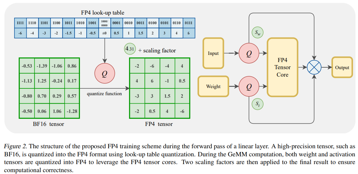
Forward pass : At every training steps, during the forward pass the weights are quantized to FP4 and the conventional operations are held to compute output. For the quantization they used conventional ABSMAX function which simply put is projecting each value to its nearest largest value in the matrix (similar to our how to quantize section). This quantization also includes quantization of activations, which is tricky hence explained in greater detail in next block.

Equation of ABSMAX Backward pass : The gradients are computed on FP4 but instead of applying it directly to the child network (which will result in loss of information) they convert gradients back to fp16 precision (using DGEs, this we will discuss next) and then apply it on master network, which leads to more information preservation. Once, the fp16 weights are updated, they are again requantized into fp4 using same ABSMAX function, and this process is repeated till convergence.

Now we know how the training loop looked like, let's discuss some internal components as well.
Quantizing activations
As activations are computed on the fly during forward pass because they are function of weights (already Quantized) and inputs (generally normalized), converting them to FP4 becomes challenging.
But, why to even convert them to FP4, why not just use them as it is?One reason why one would look for quantizing activations is because activations are also very memory intensive during training (backpropogation). It scales even more with batch size.
Another reason is compatibility. Think it like this, Imagine you have two rulers, One marked in millimeters (FP16) and the other marked in centimeters (FP4). Trying to measure and compare using both at once is awkward and imprecise. You’ll get rounding errors and misalignment. It’s better to convert everything to a common scale before operating. Hence, the answer lies in overflow due dtype incompatibility. Imagine multiplying a fp4 (weights) and activation/output from previous layer (unknown precision). This will result into:Precision Mismatch Causes Overflow:
Multiplying low-precision weights (like FP4) with higher-precision activations (like FP16) can cause overflow or underflow due to incompatible dynamic ranges. This leads to inaccurate or unstable results.Hardware Requires Uniform Formats:
Specialized hardware (like tensor cores or AI accelerators) is optimized for operations where both inputs are in the same precision. Mixing types leads to inefficient computation or unsupported execution.
Hence, we need the quantization part, but, how did the authors do it?
Activations in general have quite wide range due to outliers (see the graph below)
These outliers makes it hard to quantize as they lie on really large range, resulting in a lot of information loss while quantizing. As the number of bins are fixed and they stretch the value range, forcing quantizers to spread fixed bins (like in a lookup table) across a large span (larger value range per bin). This results in poor resolution for the dense central region where most values lie.
Example:
Imagine your lookup table has only 16 bins (as in FP4). If one activation spikes to 100 while most values are between -1 and 1, the bins must stretch from -100 to 100. That means most of the bins cover huge value intervals, and subtle variations in the majority of activations are lost—leading to degraded performance.
This is why techniques like clipping, log-scaled quantization, or per-channel quantization are often used to tackle those outliers and preserve useful information within a fixed bin budget.
In paper, authors followed the similar route. They calculated the top 0.1% of the activations and treated it as threshold. Any value above this threshold is clamped, this narrows the range as outliers are now out of the picture. Now, when ABSMAX is applied it results in much smoother and verbose activations. The clamped values/residue are not removed as they do have information, and are hence stored in a spare matrix which is then added separately in fp16 precision onto next layers activation. This is much better as firstly, it's addition (less number of read/writes) and secondly the matrix is sparse (mostly zeros hence less GPU read/write ops) and hence less value to work with.
De-Quantization of values back to FP16 using DGEs
As we discussed above the ABSMAX function is non-differentiable, hence, computing The gradients becomes a huge problem. See why differentiability is important for backward pass here.
To handle this, conventionally, it is assumed that the values after and before quantization would remain more or less same, hence, the values/gradients are computed/used as it is, this is called as STEs (Straight Thorough Estimators). But, this over-simplistic assumption leads to significant information loss and error accumulation resulting in unstable training.
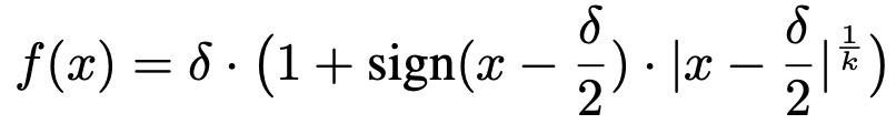
To tackle this, authors proposed DGEs (Differentiable Gradient Estimators). The process is simple, forward pass remains as it is, but while backward pass, they used a continuous approximation of original quantized function (see the image below)
notice the tiny nudge to induce continuity Let's go through the formulation, here:

𝑓(𝑥)≈quantized(𝑥), but is smooth enough to allow gradients δ is the quantization step size (the interval between quantized levels)
𝑘 controls how "sharp" the function is (higher 𝑘 → closer to real quantization)
The sign term ensures the curve bends differently on either side of the midpoint
This derivative varies with x, unlike STE’s flat/zero gradient, making it more reflective of actual quantization behavior. As K goes to infinity the function tends to the actual quantization function, but if it goes to 0 or is a small number then it becomes a smooth approximate, which is the property we need for proper gradient computation.

observe the constant and 0 gradients for STE and Hard quantization, notice that DGE has informative/non-zero gradients It's like adding your discrete (non-continuous) signal which in our case is ABSMAX quantized weights to a continuous signal (not exactly, as the addition operation doesn't guarantee a continuous signal as output, hence the formulation above, but you got my point) or smoothening/moving average. This formulation helps in providing a directed guidance to the gradient computation while preserving all the required complexity.

adding two signals, in this image both are continuous, but in paper the green signal is discrete (but, I hope you got my point)


Results/outcomes
Model & Setup: LLaMA 2 was trained from scratch on the DCLM dataset across various precisions, using identical hyperparameters. FP4-specific tweaks included k=5 for gradient estimation and α=0.99 for activation clamping.

Training Comparison: FP4 achieved training loss very close to BF16 across model sizes (1.3B–13B). Despite slightly higher loss, FP4 held up well even on downstream zero-shot tasks.

Ablation Studies: On a smaller 1.3B model trained with 10B tokens, FP4 with proper techniques (DGE + OCC) matched FP8 baselines, while direct FP4 (W4A4) lagged significantly.
Weight Quantization: Directly quantizing weights to 4-bit (W4A8) caused minimal loss, showing weights are easier to compress. DGE further improved convergence.

Activation Quantization: Activations are harder to quantize due to outliers. Direct FP4 (W8A4) caused NaNs; using OCC stabilized training. α = 0.99 was optimal for balancing accuracy and cost.
Granularity: Coarse quantization (tensor-wise) failed for FP4. Fine-grained vector-wise scaling (channel-wise for weights, token-wise for activations) improved accuracy, aligning better with matrix multiplication logic.


Thoughts
DGEs : Through and through, I liked the whole setup and workarounds/formulation which authors provided and I hope to see better variants/maybe trainable/hyper-network variants of this in upcoming future.
Matrix Lookups & AlphaTensor: FP4 training is deeply aligned with the idea of learning efficient matrix multiplications, as shown in DeepMind’s AlphaTensor. Since most LLM operations are matmuls, learning optimal patterns in low precision can bring huge efficiency gains.

Lack of Native FP4 Hardware : As mentioned in the paper, current GPUs lack FP4 Tensor Cores, meaning all FP4 experiments run via simulation, adding overhead due to casting and limiting actual performance benchmarks. True gains in speed and energy remain theoretical for now (though authors tried to simulate process).
Precision vs Range Tradeoff: FP4 offers compactness but struggles with outlier handling, especially in activations. Techniques like clamping and sparse residuals helps, but FP4 still has possibility of underflow and loss of dynamic range.
Quantization isn't Plug-n-Play: Training in FP4 requires careful handling of rounding, overflow, and outlier compensation. Unlike post-training quantization, it demands rethinking optimizers, learning rate scaling, and numerical stability throughout.
Future Potential : FP4's true potential lies in hardware support — custom ASICs or next-gen GPUs with native FP4 could make training faster and greener. Until then, it's a research playground with promising but unverified real-world benefits.

Conclusion
In this really long article, we started from very basics of precision and data-types, where we discussed things like Exponent, Mantissa, etc. From there we turned into answering few fundamental questions like how playing with these precision helps in training? How does error accumulation happens? Then we pondered over the ideal situation for handling these issues and also talked about a generic way to do it. From there we walked into methodology section where we discussed about the overall process and then advancements suggested by the authors to facilitate in the process. We finally discussed the outcomes and eventually what I personally think about the work.
With this we come to the end of the article. I hope this article provided the necessary support and framework for you to start reading more about this topic. In no ways, my article is 100% correct or complete, I have omitted a lot of nuances and details to fit this in one readable and engaging blog.
I will encourage you to refer to the paper and go through the references in great details to have more fine-grained understanding.
Paper link : https://arxiv.org/abs/2501.17116
That's all for today.
Follow me on LinkedIn and Substack for more such posts and recommendations, till then happy Learning. Bye👋