Building AI agents to play video games

How did humans build agents which can play video games?

Let us go back in history to explore.

We are in the year 1972. A lot of things happened this year. The Godfather movie premiered, which was a landmark in film history, NASA launched Apollo 16 and Apollo 17 missions and the first scientific pocket calculator was released.

Amidst all this, there was another development.

The first arcade-based video game was released. It was called as Pong.

If you see closely, you can see that there are two paddles on the screen which are controlled by two players. The goal is to move the paddle up and down to move the ball past the opponent's paddle.

The game of Pong was special because it was the first commercially successful video game and marked the true beginning of the video game industry.

But these units were very big and not available to people at homes.

Until microprocessors became available in 1975.

In 1975, Atari released Pong. It was a self-contained unit - just plug it into the TV and play. It sold over 1 lakh 50 thousand units in the first year, becoming a holiday sensation in the US. This made home gaming mainstream.

2 years later, in the year 1977, the Atari 2600 was released. Instead of being limited to one game like Pong, it could now be put in 7 different game cartridges. This console brought popular games like Space Invaders, Pac-Man, and Asteroids.

We started by playing video games in arcades, and then moved to playing video games at our houses. What's next?

The next revolution happened after 36 years.

In 2013, Google DeepMind released a paper where they showed AI can be trained to play Atari 2600 games. And they used Reinforcement learning.

In this post, we will understand and learn how to train an AI agent to play video games.

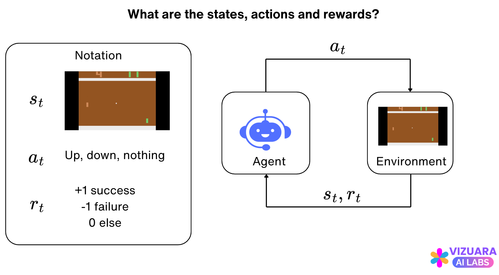
First, let us recap a little bit about the values of states.

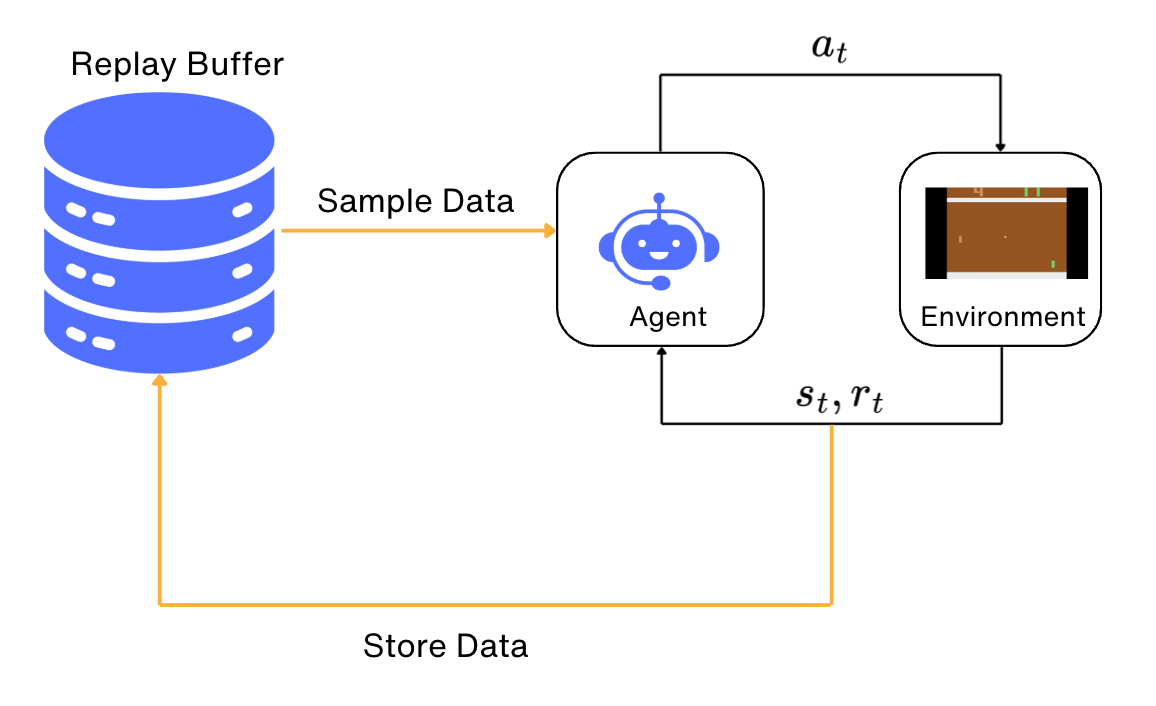
Reinforcement learning problems are traditionally modeled as agent-environment interfaces which look like these:

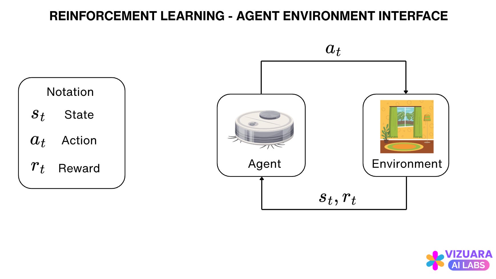
The agent receives states or observations from the environment, takes an action based on those observations, and then receives rewards from the environment.

The main task of Reinforcement Learning is to develop a policy which can tell the agent which actions to take for all the states which the agent encounters.

Now, to understand which action to take in every state, we focus on the long-term returns from that state instead of the immediate reward.

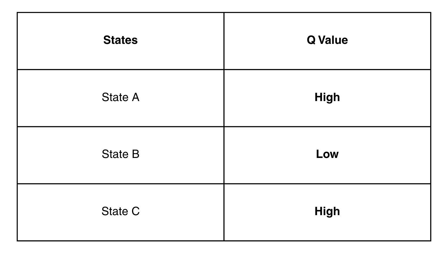
This long-term return is also called the Q-value.

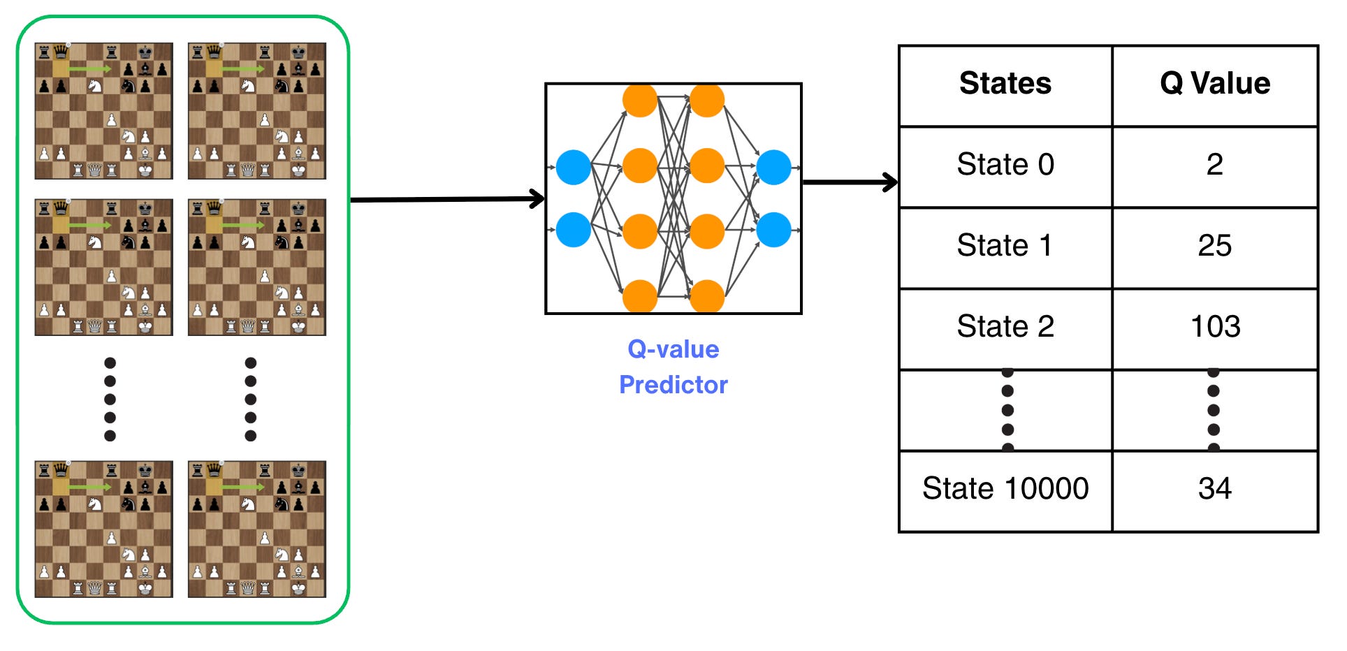
What we do is, for every state, we build a table which consists of the Q-values estimated for each state.

Till 1990s to 2000s, people used long tables to represent the Q-values. The table looked like follows:

Now, this table is continuously improved by using different methods, such as the three horsemen of classical reinforcement learning which we discussed in the last lecture: Dynamic programming, Monte Carlo and Temporal difference methods.

One problem with maintaining tables is that the size of the table increases with the number of states.

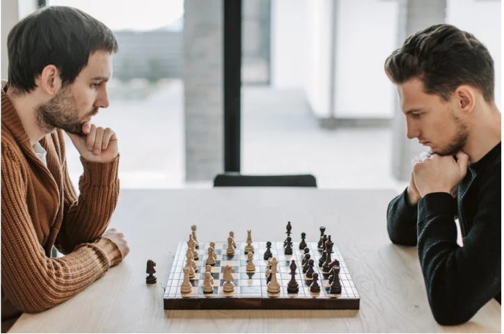
For example, the game of chess has 10^44 possible states. For each state, there are dozens of possible actions. It would take billions of years to store all the key values in a table.

But there is a workaround to this. In fact, this problem is the main reason why the field of machine learning was born.

The main question we ask is: "Can we store the Q-values for some states and approximate to others?"

This is exactly what functional approximation methods do.

Taking the game of chess as an example. The question we are asking is: Can we use 10,000 states for training the Q-value function and then use the game model to predict the Q-values for other states?

Using a neural network.

Something like this:

Looks quite cool, but…

Will this actually work?

Will a neural network learn to generalize to unseen data on such problems which require complex planning?

People did not trust these function approximation methods.

Until 1992…

In 1992, TD-Gammon was developed. It was the first program to reach a near-world-class level in complex games such as backgammon using self-play and learning from experience.

It was developed by Gerald Tesauro at IBM in 1992, and it used function approximate methods - it used neural network to predict the Q-values.

This was a very big deal, because in 1992, deep learning was not even developed. It was long before deep learning became popular in early 2010.

People had given up hope on neural networks, and this achievement revived the interest in both neural networks and reinforcement learning.

By 2013, we had good enough computing power to have deep neural networks. AlexNet had come out in the previous year which was a ground-breaking convolutional neural network that achieved significant success in image recognition and is known for its deep architecture.

So it makes sense that around the same time when Deep Learning was gaining popularity, DeepMind applied these deeper networks to explore problems using Reinforcement Learning methods.

Learning to Play the Game of “Pong” with Reinforcement Learning

First, let us understand the game of Pong through the lens of the agent-environment interface as typically defined in reinforcement learning problems.

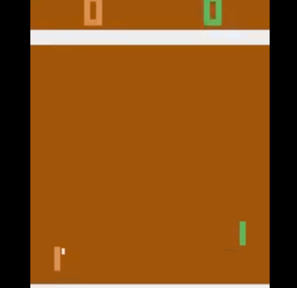
Let us look at a single frame encountered while playing the game of Pong. Here, we represent the green paddle, the opponent represents the brown paddle, and the white dot represents the ball which is moving in the environment.

Our task is to not allow the ball to get past our paddle and to do that we can move the paddle up or down when the ball approaches our side of the environment. When the ball is on the other side, on the other half of the environment, we can choose not to do anything.

From this description, you probably might get an idea of the states and the actions for the Pong environment.

The states are simply the Pong game frames. A single frame consists of an array of pixels with 210 rows and 160 columns. The pixelated image (state) might look something like this:

Pixellated versions of images have always baffled me, and the way machine learning systems predict the type of the image simply from the pixels (as in image recognition tasks) looks like an astonishing feat, and I am always amazed by how that works.

What about actions? The actions are simple, we have three actions for our environment:

1. Move paddle up

2. Move paddle down

3. Do nothing

The rewards are:

1. +1 if the agent successfully hits the ball past the opponent's paddle

2. -1 if the agent misses the ball

3. 0 for all other frames

The agent-environment interface diagram looks as follows:

Policy:

Now that we have defined the states, actions and rewards, we can move on to finding an optimal policy which maximizes our chances of winning the game of Pong.

Let us think about the possible methods we can use and through the process of elimination select the right method.

First, Dynamic Programming. For dynamic programming, we need a complete model of the environment. I have no idea what are the probabilities of transitioning from one state to another in the game of Pong. This completely rules out the option of dynamic programming.

Next, Monte Carlo Methods. Well, this is better than dynamic programming because I do not need a model of the environment. I can simply collect a lot of experiences and update my predictions about action values for all states and actions. The problem with Monte Carlo methods is that, I need to wait till the end of the episode before I make any updates. This will be very time-consuming, and it rules out the option of Monte Carlo methods.

What about temporal difference methods, especially Q-learning? Q-learning does not require a model of the environment and also it updates the action values immediately after taking a step in the environment.

This sounds great until we hit a roadblock! The way we have defined the states for the Pong environment, there are 10^70,802 possible states for the environment. It is impossible for us to store a Q-table which has all these values.

So we need to use function approximation methods.

More specifically, we need to use a neural network, which can map the states and actions onto a value. Using a deep neural network is one of the most popular options, especially when dealing with observations represented as screen images.

Let us look at the usual Q-learning algorithm and the modified Q-learning algorithm using a deep neural network.

Conventional Q-Learning Algorithm:

Step 1: Start with an empty table for Q(s,a)

Step 2: Obtain s,a,r from the environment using the ε-greedy policy

Step 3: Obtain a' using greedy policy

Step 4: Make a Bellman update according to the following equation:

Q(s,a) = Q(s,a) + ⍺(r+ƔmaxQ(s',a'))

Step 5:Repeat from Step 2 until converged

This is also called as tabular Q-learning.

Modified Q-learning Algorithm:

In the modified Q-learning algorithm, the Q-values are not updated through the Bellman equation, but rather the weights of the neural network that represents the Q-values are updated using the Stochastic Gradient Descent algorithm.

The algorithm looks as follows:

Step 1: Initialize Q of s, a with some initial approximation 

Step 2: By interacting with the environment, obtain the tuple (s,a,r,s')

Step 3: Calculate Loss - (Q(s,a)-(r+ƔmaxQ(s',a'))^2

Step 4: Update Q(s,a) using the stochastic gradient descent algorithm by minimizing the loss with respect to the model parameters.

Step 5: Repeat from Step 2 until converged. 

Here you might have noticed something strange. The target for our neural network is related to our neural network itself.

This is something we never do in supervised or unsupervised learning categories of machine learning problems.

Don't worry about the neural network architecture for now. Focus on how the loss is calculated by using the same network twice.

Since this architecture involves deep neural networks, this algorithm is also called Deep Q-Networks (DQN).

Unfortunately, this algorithm does not work very well.

Let's see why:

(1) Interaction with the environment

If our representation of Q is good, then the experience that we get from the environment will show the agent relevant data to train on.

However, we are in trouble when our approximation is not perfect. The beginning of the training, for example. In such a case, our agent will be stuck with bad actions for some states without ever trying to behave differently. This is the Exploration vs Exploitation dilemma.

On one hand, our agent needs to explore the environment to build a complete picture of transitions and action outcomes. On the other hand, we should use interaction with the environment efficiently. We should not waste time by trying actions that we have already tried and learned outcomes for.

Method that performs such a mix of two extreme behaviors is known as epsilon-greedy method. I have actually included this, while describing the algorithms in the code blocks above.

(2) Stochastic Gradient Descent Optimization

One of the fundamental requirements for stochastic gradient descent optimization is that the training data is independent and identically distributed (i.i.d), which means that our training data is randomly sampled from the underlying dataset we are trying learn on.

In our case, this criterion is not fulfilled because our samples are not independent; they will all be very close to each other as they will belong to the same episode.

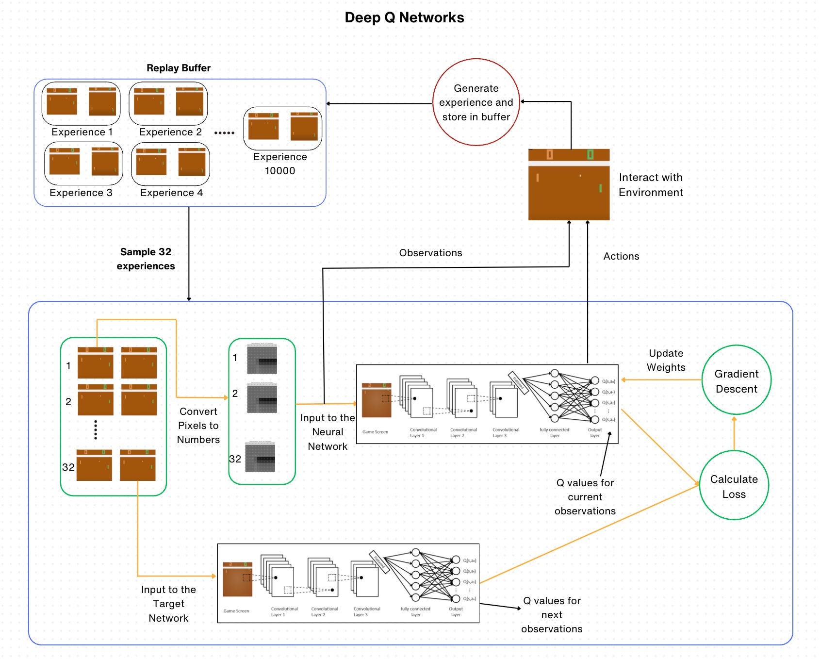
To deal with this, we usually use a large buffer of our past experience and sample training data from it, instead of using our latest experience.

This technique is called a replay buffer.

The replay before allows us to train on more or less independent data.

You can imagine some other applications where replay buffers would be useful. For example, in language models, the states are the tokens which are written as a response to a prompt. These tokens are related to each other. Replay buffers allow us sample tokens which are independent of each other.

(3) Correlation between steps

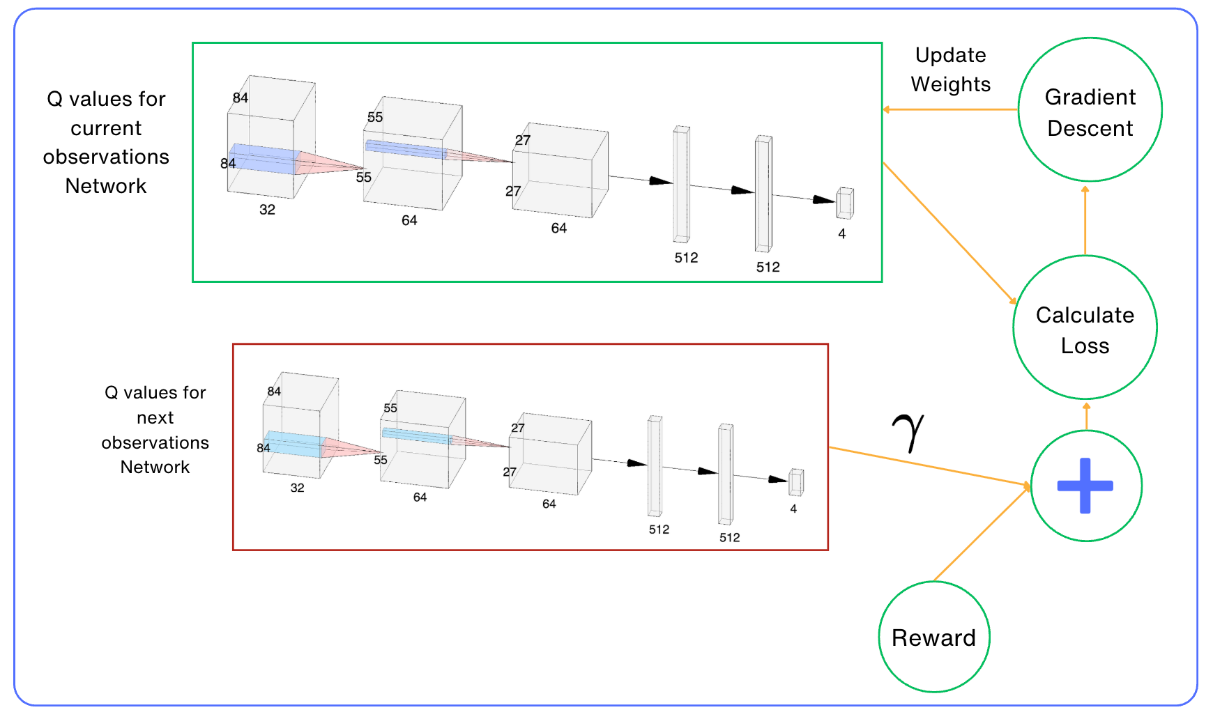
You would have noticed that we are using the same neural network to calculate the Q-values of the current state and the next state, which is used to calculate the target.

This makes them very similar, and it is very hard for neural networks to distinguish between them.

When we perform an update of our neural network's parameters to make Q(s,a) closer to the desired result, we can indirectly alter the values produced for Q(s', a') and other states nearby.

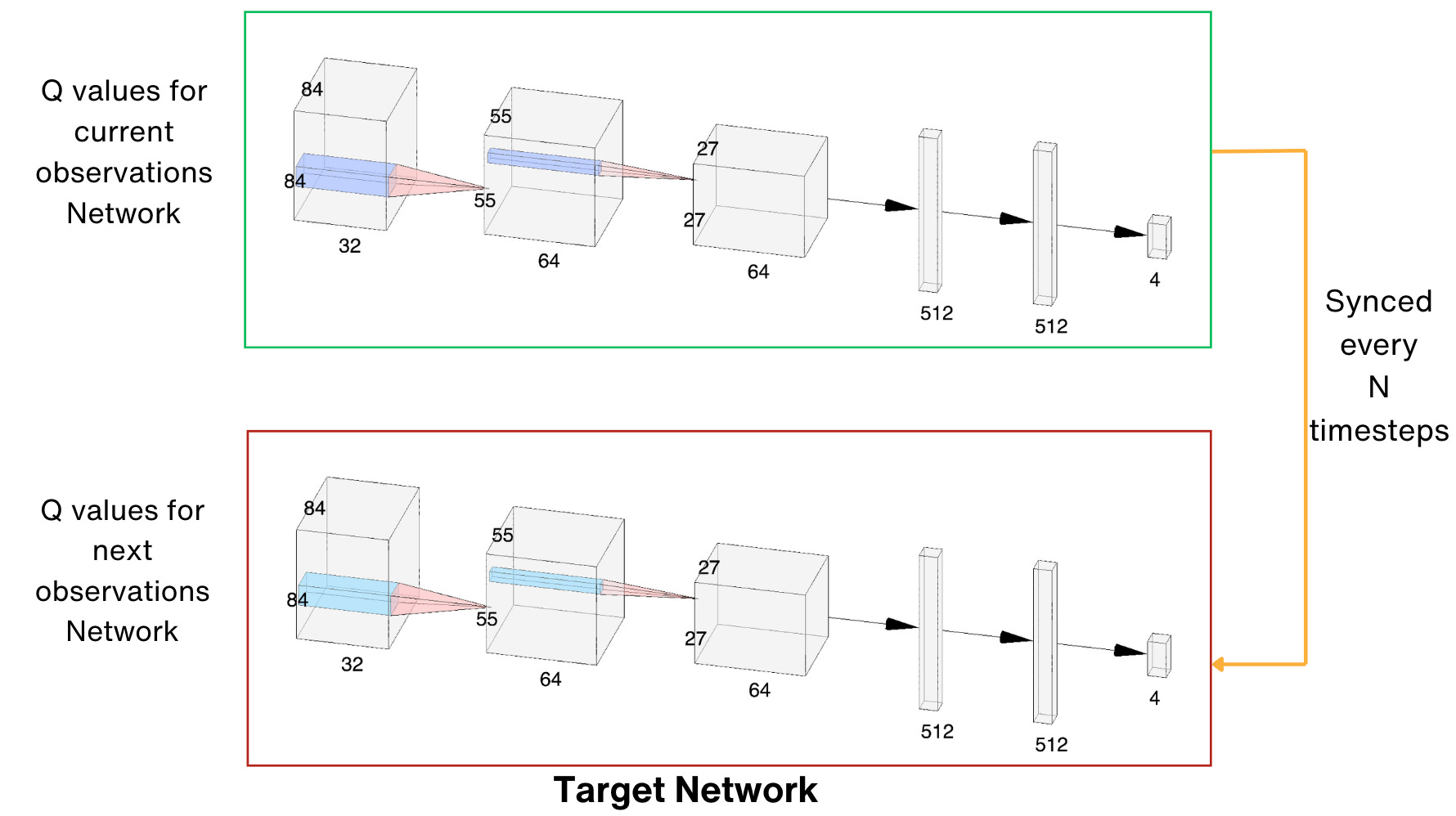
This can make our training very unstable, like chasing our own tail. When we update Q (s,a), then we will discover that Q(s', a') becomes worse, but attempts to update it can spoil our Q(s,a) approximation even more, and so on.

To make the training more stable, there is a trick called Target Network by which we keep a copy of our network and use it for Q(s', a') value. This network is synchronized with our main network only periodically, for example, once every n steps (such as 1000 or 10,000 training iterations) and is usually quite a large hyperparameter.

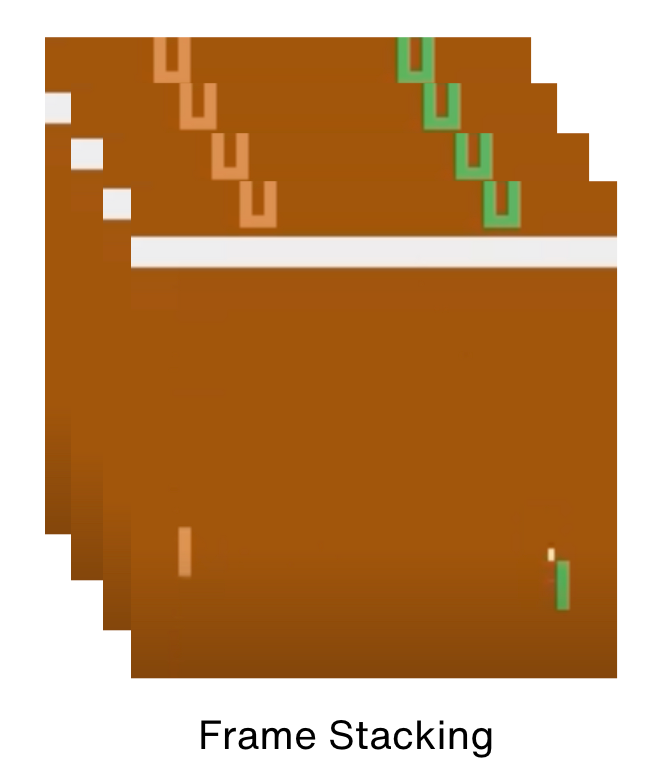
(4) The Markov Property

The strategy for the game of Pong does not only depend on the current observation but we have to look at a sequence of observations which have happened in the past. For example, if the ball is in the middle of the screen, it might mean that it is either moving towards you or away from you.

This means that the state signal does not satisfy the Markov property.

For the Bellman equation to work, Markov assumption is fundamental. There is a small technique to push our environment back into the MDP domain. The solution is to maintain several observations from the past and use them as a state. In the case of Atari games, usually k subsequent frames are stacked together and used as an observation. The classical number of k for Atari is 4.

It is through a combination of epsilon-greedy, the replay buffer, target network, and stacking of frames that DeepMind was able to successfully train a neural network on a set of Atari games, demonstrating the efficiency of this approach when applied to complicated environments.

Final DQN Algorithm:

Step 1: Initialize parameters for Q(s,a) and Q^(s,a) with random weights,ε=1 and empty the replay buffer.

Step 2: With probability ε, select a random action a; otherwise, a=argmax Q(s,a).

Step 3: Execute action in an emulator and observe the reward (r) and the next state (s').

Step 4: Store the transition (s,a,r,s'), in the replay buffer.

Step 5: Sample a random mini-batch of transitions from the replay buffer. 

Step 6: For every transition in the buffer, calculate the target:
Target = r+ƔmaxQ^(s',a').

Step 7: Calculate the loss: (Q(s,a)-Target)^2.

Step 8: Update Q(s,a) using the SGD algorithm by minimizing the loss with respect to the model parameters. 

Step 9: Every N steps. copy weights from Q to Q^.

Step 10: Repeat from step 2 until converged.

Playing Atari games using our policy

Let us first design our neural network.

The DQN Model:

The model published in Nature has three convolutional layers followed by two fully connected layers. All layers are separated by rectified linear unit non-linearities.

The model looks as follows:

The output of the model is Q-values for every action available in the environment.

The code for the model looks as follows:

class DQN(nn.Module):
    def __init__(self, input_shape, n_actions):
        super(DQN, self).__init__()

        self.conv = nn.Sequential(
            nn.Conv2d(input_shape[0], 32, kernel_size=8, stride=4),
            nn.ReLU(),
            nn.Conv2d(32, 64, kernel_size=4, stride=2),
            nn.ReLU(),
            nn.Conv2d(64, 64, kernel_size=3, stride=1),
            nn.ReLU(),
            nn.Flatten(),
        )
        size = self.conv(torch.zeros(1, *input_shape)).size()[-1]
        self.fc = nn.Sequential(
            nn.Linear(size, 512),
            nn.ReLU(),
            nn.Linear(512, n_actions)
        )

    def forward(self, x: torch.ByteTensor):
        # scale on GPU
        xx = x / 255.0
        return self.fc(self.conv(xx))

The convolution part processes the input image.

The output from the last convolution filter is flattened into a 1D vector and fed into two linear layers.

The final piece of the model is the forward function which accepts the input tensor.

Performing a step in the environment:

The main method of the agent is to perform a step in the environment and store its result in the buffer. To do this, we need to select the action first. This is done by the following piece of code:

    def play_step(self, net: dqn_model.DQN, device: torch.device,
                  epsilon: float = 0.0) -> tt.Optional[float]:
        done_reward = None

        if np.random.random() < epsilon:
            action = env.action_space.sample()
        else:
            state_v = torch.as_tensor(self.state).to(device)
            state_v.unsqueeze_(0)
            q_vals_v = net(state_v)
            _, act_v = torch.max(q_vals_v, dim=1)
            action = int(act_v.item())

With the probability ε, we take the random action. Otherwise, we use the model to obtain the Q-values for all possible actions and choose the best.

As the action has been chosen, we pass it to the environment to get the next observation and reward, store the data in the experience buffer, and then handle the end-of-episode situation.

This is done by the following piece of code:

        new_state, reward, is_done, is_tr, _ = self.env.step(action)
        self.total_reward += reward

        exp = Experience(
            state=self.state, action=action, reward=float(reward),
            done_trunc=is_done or is_tr, new_state=new_state
        )
        self.exp_buffer.append(exp)
        self.state = new_state
        if is_done or is_tr:
            done_reward = self.total_reward
            self._reset()
        return done_reward

Now the next step is to collect:

• States

• Actions

• Rewards

• Flags

• New states

This is important because we will use this information to calculate our loss.

This is done by the following piece of code:

def batch_to_tensors(batch: tt.List[Experience], device: torch.device) -> BatchTensors:
    states, actions, rewards, dones, new_state = [], [], [], [], []
    for e in batch:
        states.append(e.state)
        actions.append(e.action)
        rewards.append(e.reward)
        dones.append(e.done_trunc)
        new_state.append(e.new_state)
    states_t = torch.as_tensor(np.asarray(states))
    actions_t = torch.LongTensor(actions)
    rewards_t = torch.FloatTensor(rewards)
    dones_t = torch.BoolTensor(dones)
    new_states_t = torch.as_tensor(np.asarray(new_state))
    return states_t.to(device), actions_t.to(device), rewards_t.to(device), \
           dones_t.to(device),  new_states_t.to(device)

Now we are ready to define our loss function.

Defining the Loss Function

First, the action values of the current states are calculated. This is done using the following approach:

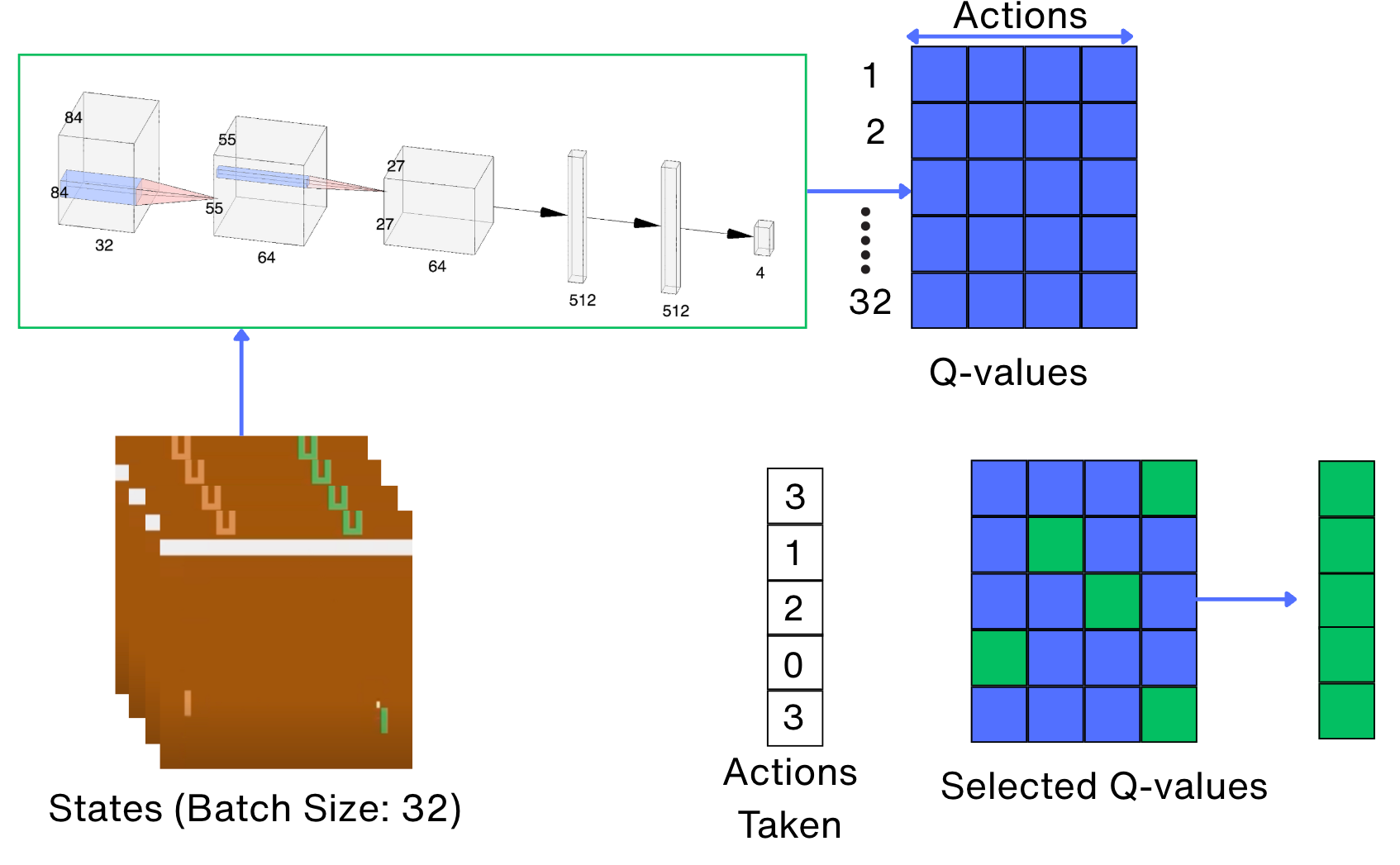
The following is the code for selecting the action values of the current states.

def calc_loss(batch: tt.List[Experience], net: dqn_model.DQN, tgt_net: dqn_model.DQN,
              device: torch.device) -> torch.Tensor:
    states_t, actions_t, rewards_t, dones_t, new_states_t = batch_to_tensors(batch, device)

    state_action_values = net(states_t).gather(
        1, actions_t.unsqueeze(-1)
    ).squeeze(-1)

Next, we calculate the action values for the next states. This is done using the following approach:

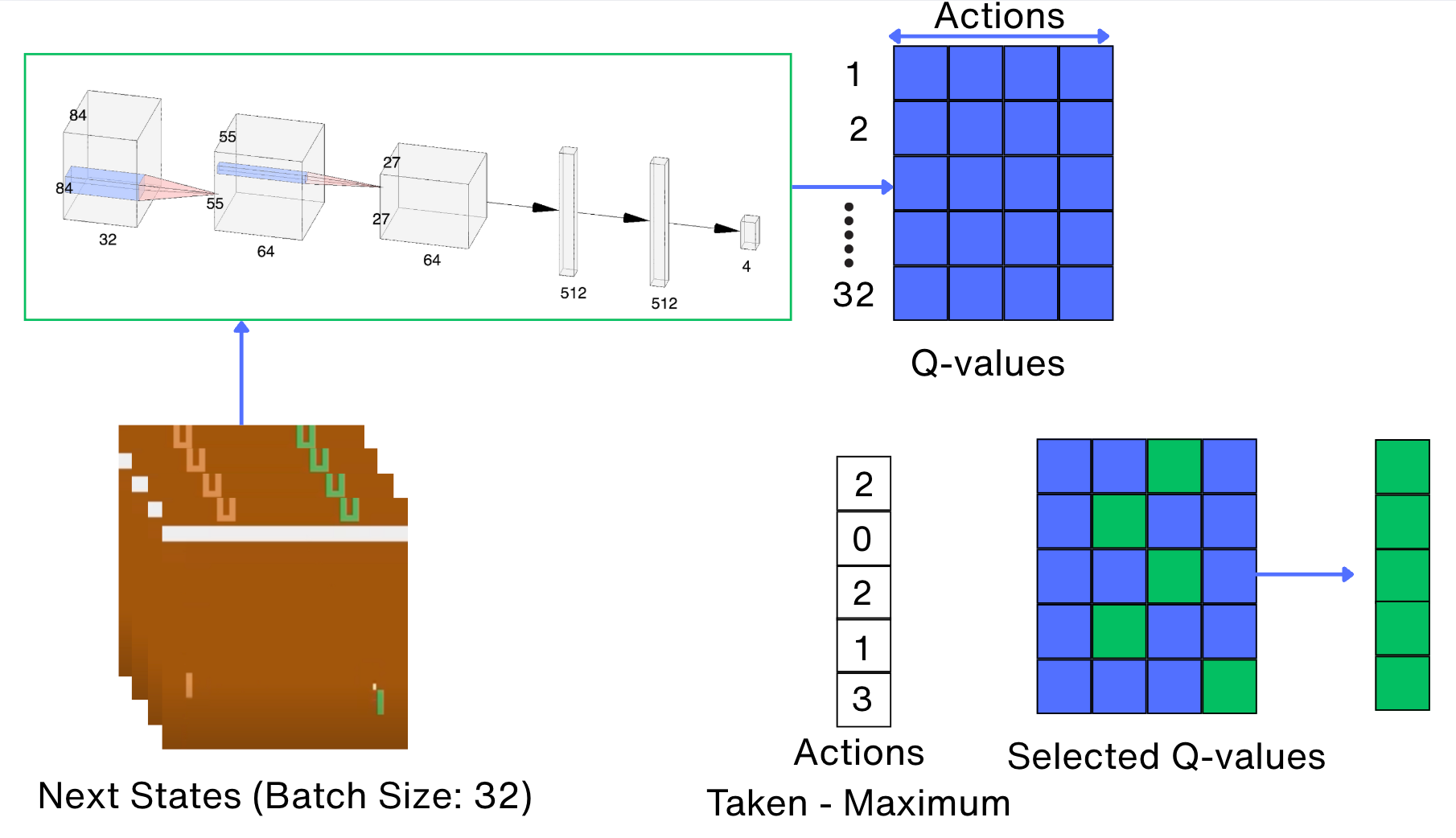
The following is the code for selecting the action values of the next states:

with torch.no_grad():
        next_state_values = tgt_net(new_states_t).max(1)[0]
        next_state_values[dones_t] = 0.0
        next_state_values = next_state_values.detach()

Now we are ready to calculate the loss:

expected_state_action_values = next_state_values * GAMMA + rewards_t
    return nn.MSELoss()(state_action_values, expected_state_action_values)

Starting the training loop:

The key portions of the training loop are:

1. Initializing the neural network that we are going to train and our target network with the same architecture.

2. Making a single step in the environment

3. Check whether our buffer is large enough for training First, we should wait for enough data to be accumulated which in our case is 10,000 transitions.

4. Sync parameters from our main network to the target network every 1000 steps.

5. Backpropagate the loss and update weight parameters

This is done by the following key lines of code:

net = dqn_model.DQN(env.observation_space.shape, env.action_space.n).to(device)
tgt_net = dqn_model.DQN(env.observation_space.shape, env.action_space.n).to(device)

reward = agent.play_step(net, device, epsilon)

if len(buffer) < REPLAY_START_SIZE:
            continue
        if frame_idx % SYNC_TARGET_FRAMES == 0:
            tgt_net.load_state_dict(net.state_dict())

optimizer.zero_grad()
        batch = buffer.sample(BATCH_SIZE)
        loss_t = calc_loss(batch, net, tgt_net, device)
        loss_t.backward()
        optimizer.step()

The final architecture for the whole process looks as follows:

That’s it!

Running our RL Agent

I ran the code for 600000 time steps, and we get a sweet reward trajectory as follows:

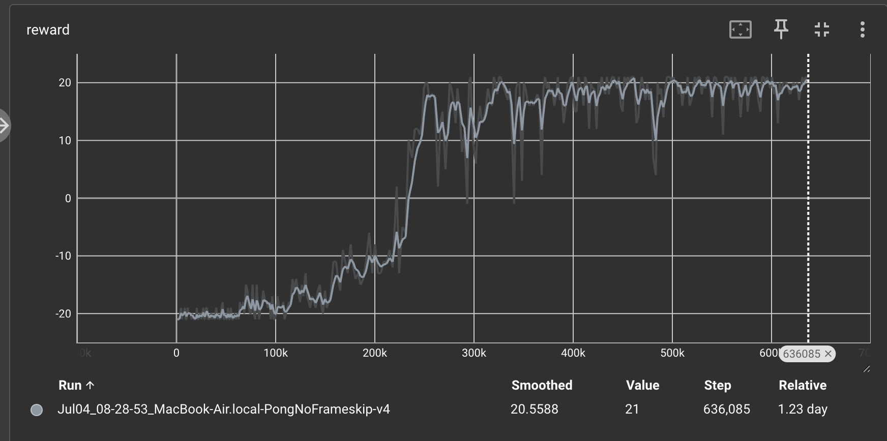
This means that our agent is learning and getting better with time.

During the first 10,000 steps, we do not do any training. Several dozen games later, our DQN agent start to figure out how to win 1 or 2 games out of 21, and the average reward begins to grow.

Finally, we get close to a reward of 20, which means that our agent is winning 20 games out of a total of 21 games.

That is indeed amazing!

Let us see some videos of how our agent performs:

Our agent starts out with not moving at all. So the action it chooses is just to not do anything, and our opponent continues to score against us.

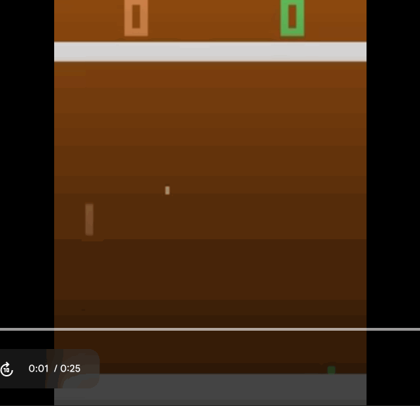
But we slowly improve with time and we learn to score past the opponent. This is how we start playing the game after 600000 time steps.

There is a sense of joy when you see your agent improve with time.

It is almost like you are teaching a kid to learn something. Initially, they are making a lot of mistakes, and finally, they are able to learn the skill.

RL-BASELINES3-ZOO

If you want to just use a pre-trained agent and see how the agent works, There is an amazing repository called RL-Baselines3-Zoo.

The goal of this repository is to make coding with reinforcement learning very easy.

It does not necessarily teach you the basics of RL and how the code works, but it is a great repo to tweak parameters and try out various algorithms and how they work for practical problems.

Using a single line of code, you can see your agent play the Pong game.

To do this, the first step is to clone the repository.

Once you have cloned the repo, run the following piece of code:

python rl-baselines3-zoo/enjoy.py --algo dqn --env PongNoFrameskip-v4

That's it.

Refer to this GitHub repo for reproducing the codes shown in this article: https://github.com/RajatDandekar/Hands-on-RL-Bootcamp-Vizuara