Decoding Convolutional Neural Networks: From Pixels to Patterns

Discover how CNNs mimic the human eye with sliding filters, learn to see features instead of just pixels, and unlock the power of image classification.

Table of content

1. Introduction: The Quest to See

2. The Problem: Why a Straight Line (of Pixels) Fails at Vision

3. The Solution: The Architecture Inspired by the Brain

4. The Strategy: The Detective and the Magnifying Glass

5. Deep Dive: The Building Blocks of a CNN

6. Putting It All Together: From Raw Image to Final Prediction

7. Going Deeper: See CNN in Action with the Vizuara AI Learning Lab!

8. Conclusion

1. Introduction: The Quest to See

Think about how you're reading this text right now. Your eyes don't process it as a meaningless collection of black and white pixels. You instantly recognize letters, which form words, which form sentences. If you look up from your screen, you might see a coffee mug, a window, or a pet. You don't consciously think, "That's a circular edge, connected to a curved handle, filled with a brown texture." You just see a mug. This ability to perceive patterns, objects, and scenes is one of the most remarkable feats of human intelligence, yet we do it effortlessly.

Now, how do we teach a machine this same intuitive ability?

In our previous posts, we taught our machine to understand relationships in numbers with Linear Regression and to classify outcomes with Logistic Regression. We even gave it a sense of language by exploring Word Embeddings and a concept of memory with Recurrent Neural Networks. But all these models have a fundamental blindness when it comes to images. An image isn't a simple line of numbers or a sequence of words. It's a rich, spatial tapestry where the arrangement of every pixel matters.

This is the next frontier in our journey: teaching our machine not just to calculate or remember, but to see. This is the quest that leads us to one of the most powerful and influential architectures in all of AI: the Convolutional Neural Network (CNN). In this post, we'll decode how CNNs are masterfully designed to think in images, moving from raw pixels to recognizable patterns, just like our own brains.

2. The Problem: Why a Straight Line (of Pixels) Fails at Vision

Alright, so we have a new mission: teach a computer to look at a picture and tell us if it's a cat, a dog, or a car. Being familiar with our previous tools, a natural first thought might be: "Why not just use what we already know? Let's take a standard neural network, like the ones we've discussed before!"

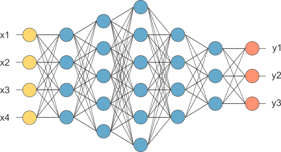
It seems logical. A computer sees an image as just a grid of numbers (pixels), right? A standard 28x28 grayscale image is just 784 pixels. Why can't we just "unroll" or "flatten" this grid into one long line of 784 numbers and feed it into our trusty feedforward network?

This is where we hit a massive, deal-breaking wall. In fact, this approach fails so spectacularly that it reveals exactly why we need a completely new kind of architecture. Here are the two fatal flaws:

1. It Destroys Spatial Structure

Imagine tearing up a photograph of a face into a thousand tiny strips and laying them end-to-end. Could you still tell it's a face? Probably not. The magic of an image isn't in the individual pixels; it's in their arrangement. An eye is an eye because of how the pixels for the pupil, iris, and sclera are positioned relative to each other.

When we flatten an image into a single vector, we throw all of this crucial spatial information into the trash. The network has no idea which pixels were neighbors. The pixel that was at the top-right corner is now just another number in a line, no different from the pixel that was in the bottom-left. It's like trying to read a book by shuffling all the words. This loss of structure makes it nearly impossible for the network to learn about shapes, textures, and objects.

2. It's Brittle and Inefficient (No Parameter Sharing)

Let's say, by some miracle, we manage to train our flattened-image network to recognize a cat in the top-left corner of our images. The network would learn that "pixels 1-50 having these specific values means there's a pointy ear here."

Now, what happens if we show it a new image where the cat is in the bottom-right corner?

To the network, this is a completely new, alien problem. The pixels corresponding to the pointy ear are now in a totally different part of the input vector (say, pixels 700-750). The network has to learn this pattern all over again, from scratch, for that new position. It has no concept of a "pointy ear" as an object; it only knows about pixel values at fixed locations. This is wildly inefficient. We want a network that learns to detect a pointy ear anywhere in the image, using the same logic (the same parameters).

This is precisely where our old tools fail us. We need a network that:

• Respects and leverages the 2D (or 3D) structure of an image.

• Learns to detect features (like edges, corners, textures) regardless of their position.

We need a network that doesn't just see a line of pixels. We need a network that learns to see.

3. The Solution: The Architecture Inspired by the Brain

So, our standard networks are blind to the very essence of an image its spatial structure. How do we fix this fundamental flaw? The answer, as is often the case in AI, comes from looking at the best image processor we know: the human brain.

In the 1950s and 60s, researchers Hubel and Wiesel conducted groundbreaking experiments that showed how the visual cortex in mammals processes information. They discovered that specific neurons in the brain fire in response to very particular features in our field of vision, like lines at a certain orientation (horizontal, vertical, diagonal). More complex neurons then combine the signals from these simpler ones to recognize more complex shapes, and so on. In essence, our brain processes visual information in a hierarchy of increasing complexity. It doesn't see a car; it sees edges, which form wheels and windows, which in turn form the object we recognize as a car.

This is the brilliant insight that led to the Convolutional Neural Network (CNN).

Instead of flattening the image and destroying its structure, a CNN is designed to work with the image in its original grid-like form. It embraces the spatial relationship between pixels. A CNN doesn't learn about individual pixels at fixed positions; it learns to recognize small, localized patterns like edges, corners, colors, and textures and it learns to recognize them anywhere in the image.

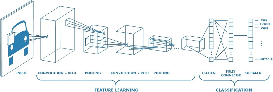
Look at that beautiful architecture. It's a pipeline designed for vision. The first part, "Feature Learning," is where the magic happens. The network scans the image to find fundamental patterns. These patterns are then used in the second part, "Classification," to make a final decision.

The core ideas that make this work are:

1. Local Receptive Fields: The network looks at the image through small windows, just like the neurons in our visual cortex respond to a small region of our visual field.

2. Shared Weights & Biases: The network uses the same "pattern detector" across the entire image. If it learns how to spot a cat's whisker, it uses that exact same detector to find a whisker anywhere, not just in one corner. This is the solution to our "brittle network" problem.

3. Hierarchical Feature Learning: The first layers learn simple features like edges. The next layers combine these edges to learn more complex features like shapes (a circle from curved edges). Deeper layers combine shapes to learn about objects (a wheel from a circle and spokes).

This is the fundamental shift. We're moving from a model that is blind to space to one that is built to understand it. But how does it actually do this? How does it "scan" the image for patterns? This brings us to the core mathematical operation of a CNN and our master analogy for understanding it.

4. The Strategy: The Detective and the Magnifying Glass

We've established that a CNN's superpower is its ability to find local patterns anywhere in an image. But what does this process of "finding a pattern" actually look like? Let's ditch the abstract jargon for a moment and use a powerful analogy.

Imagine you are a detective, and an image is your crime scene. You're not looking for one specific thing; you're looking for different types of clues. You have a set of specialized magnifying glasses.

• One magnifying glass is built to highlight vertical lines.

• Another is designed to spot horizontal lines.

• A third one is tuned to find sharp corners.

• And so on...

Each of these magnifying glasses is a Filter (sometimes called a Kernel). A filter is just a small matrix of numbers, typically 3x3 or 5x5. The specific arrangement of numbers in the filter defines what kind of clue it's looking for.

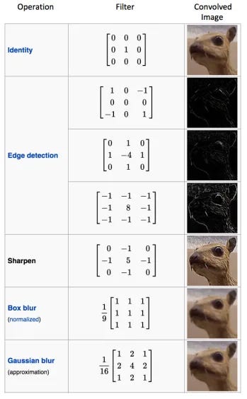
This table is incredible. It shows you exactly what I mean. A matrix like [[1, 0, -1], [1, 0, -1], [1, 0, -1]] isn't just random numbers; it's a meticulously crafted tool for detecting vertical edges. But in a CNN, we don't hand-craft these filters. The most amazing part is that the network learns the optimal values for these filters on its own during the training process! It figures out which clues are most important for solving the case (e.g., classifying an image as "cat" or "dog") and creates its own perfect set of magnifying glasses.

So, how does the detective use one of these magnifying glasses? They don't just stare at the whole crime scene at once. They perform a Convolution.

The detective takes their first magnifying glass (let's say, the one for vertical edges) and starts at the top-left corner of the crime scene (the image). They lay the glass over a small patch of the image that's the exact same size as the glass (e.g., a 3x3 patch). They then perform a special calculation: they multiply each number in their magnifying glass with the corresponding pixel value it's covering, and then sum up all the results.

This single final number is a score.

• A high positive score means the patch of the image under the glass looks very much like the feature the glass is designed to find. A "strong match!"

• A score near zero means there's not much of a match.

• A high negative score could mean it's the opposite of the feature.

The detective writes this score down in the first cell of a new, blank notepad. This notepad is our Feature Map or Activation Map. It's a map that will show us where in the image the clue was found.

Then, the detective slides the magnifying glass one pixel to the right and repeats the exact same process, calculating a new score and writing it in the second cell of the notepad. They continue this, sliding the glass across the entire image, from left to right and top to bottom, filling out the feature map with scores.

This entire process of sliding a filter over an image and calculating the scores is the Convolution Operation.

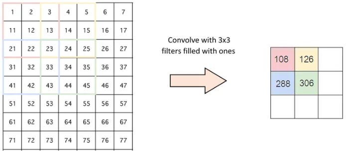
Let's visualize this with numbers.

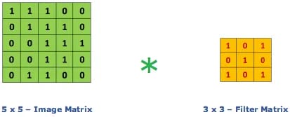
Look closely at that animation. The orange 3x3 filter is our "magnifying glass." It lays over the top-left 3x3 section of the green "image matrix."
The calculation is an element-wise multiplication followed by a sum:
(1×1) + (1×1) + (0×1) + (0×0) + (1×1) + (1×1) + (0×1) + (0×0) + (1×1) = 4

That score, 4, is recorded in the top-left of the output "Convolved Feature." This value of 4 tells us that this specific filter found a "strong" match in that location. The network then slides the filter one step to the right and does it all over again. The resulting feature map is a summary of the image, but instead of pixel values, it contains information about the location and strength of a specific feature.

Our detective analogy is holding up well, but real-world crime scenes and images are rarely simple black-and-white affairs. They have depth and complexity. Let's upgrade our understanding to see how CNNs handle this.

Seeing in Color: Convolution in 3D

So far, we've pretended our image is a flat, 2D grid (grayscale). But most images are in color. A standard color image has three channels: Red, Green, and Blue (RGB). You can think of this not as a single flat square, but as a stack of three squares.

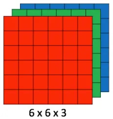
So, our image isn't just height × width; it's height × width × depth (where depth is 3 for an RGB image). How does our magnifying glass handle this?

Simple: the magnifying glass also has to have the same depth! Our filter is no longer a flat 3x3 matrix; it's a 3x3x3 cube of numbers. It's designed to look for patterns across all three color channels simultaneously.

When the 3x3x3 filter is laid over a 3x3x3 patch of the image, the convolution operation is almost the same, but with an extra dimension. It performs the element-wise multiplication and sum for the Red channel, does the same for the Green channel, and the same for the Blue channel, and then adds all three of those results (plus a single bias term) together.

This is a crucial point: no matter the depth of the input image or the filter, they always produce a 2D Feature Map. Each filter, even a 3D one, is designed to look for only one type of feature. To find multiple features, we simply use multiple filters. If we apply 32 different filters to our input image, we will get 32 different 2D feature maps stacked on top of each other, creating a new volume of height × width × 32.

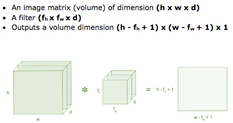
This diagram perfectly summarizes the math. Notice how the input depth d and the filter depth d must match, and the output depth is always 1 (for one filter).

Taking Bigger Steps: Strides

Our detective has been meticulously sliding their magnifying glass one pixel at a time. This is called a Stride of 1. But what if they're in a hurry or want a broader overview? They could take bigger steps, skipping over some pixels.

A stride of 2 means sliding the filter two pixels to the right after each calculation. A stride of 3 means sliding it three pixels.

Stride of 2 Pixels

What's the effect of a larger stride? The output feature map becomes smaller. This is a powerful tool for shrinking the dimensionality of our data as it flows through the network, reducing computational cost.

Handling the Edges: Padding

There's a subtle problem we've been ignoring. When we place a 3x3 filter over a 5x5 image, it can only be centered on the internal 3x3 pixels. The pixels on the very edge of the image never get to be in the center of the filter's view. This means we're throwing away information from the borders! It also causes the feature map to shrink at every layer.

The solution is simple and elegant: Padding.

Before we perform the convolution, we can add a border of zeros around the entire input image. This is called zero-padding. If we add a 1-pixel border of zeros to our 5x5 image, it becomes a 7x7 image. Now, when we slide our 3x3 filter, we can center it perfectly on every single pixel from the original image, and the output feature map will be the exact same size as the original 5x5 image.

There are two common types of padding:

• Valid Padding: This means no padding. The output shrinks, and some edge information is lost. This is the default in many libraries.

• Same Padding: This means adding just enough zero-padding so that the output feature map has the same height and width as the input image. This is extremely useful for building very deep networks without having the data dimensions shrink to nothing.

With filters, strides, and padding, we now have a complete toolkit for the convolution operation. We have our specialized magnifying glasses, we know how to use them on color images, we can control how big our steps are, and we know how to handle the edges of the crime scene. Our detective is ready for anything.

5. Deep Dive: The Building Blocks of a CNN

Our detective has successfully swept the crime scene with their collection of magnifying glasses (filters), producing a stack of Feature Maps. Each map is a grayscale image that highlights where a specific feature like a vertical edge or a particular curve was found. But this is just the first step. To build a truly powerful vision system, we need to process these maps further. This is where the other key layers of a CNN come into play.

a. The Activation Layer (ReLU): Introducing Non-Linearity

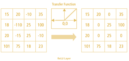
After each convolution operation, we apply an activation function to the feature map. In modern CNNs, the go-to choice is the Rectified Linear Unit, or ReLU.

The job of ReLU is incredibly simple: it looks at every single number (pixel) in our feature map and replaces all the negative numbers with zero. That's it.

output = max(0, input)

It seems almost trivial, but this step is absolutely critical. Without an activation function like ReLU, our entire network would just be a series of linear operations (matrix multiplications and additions). A stack of linear operations is, mathematically, still just a single linear operation. It would be like having a fancy calculator that can only do addition; it doesn't matter how many times you add, you can't perform more complex calculations like exponents or roots.

The real world is not linear. The relationship between pixels that form a "cat" is incredibly complex and non-linear. By introducing ReLU, we give the network the ability to learn these complex, non-linear relationships. It allows the outputs of our feature detectors to be selectively "activated" (if the feature is strongly present, resulting in a positive value) or "deactivated" (if the feature is absent, resulting in a zero). This selective firing is what allows the network to combine features in sophisticated ways in later layers.

b. The Pooling Layer: Summarizing the Evidence and Becoming Robust

After passing through the ReLU activation, our stack of feature maps is often fed into a Pooling Layer. If the convolution layer is about finding features, the pooling layer is about summarizing them.

Imagine our detective has a map with little red flags everywhere a specific clue was found. Instead of showing this highly detailed map to the chief, they might draw a grid over it and, for each grid square, just report whether any flag was found in that square. This gives the chief a downsampled, high-level summary that still contains the most important information (the presence of the clue) but is much smaller and easier to process.

This is exactly what the pooling layer does. The most common type is Max Pooling.

The network slides a small window (usually 2x2) over each feature map. Unlike the convolution's sliding window, this one has no weights to learn. It simply looks at the numbers inside its window and picks the largest one, the maximum value.

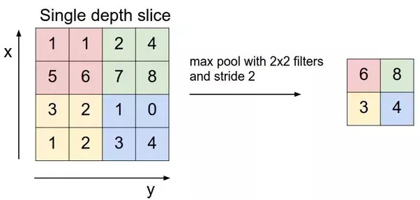
Look at the example. The 2x2 window slides over the top-left quadrant ([1, 1], [5, 6]). The maximum value is 6, so that's the output. It then slides to the next quadrant ([2, 4], [7, 8]), and the max value is 8. This process dramatically reduces the size of the feature map. A 24x24 feature map becomes a 12x12 feature map.

This has two incredible benefits:

1. Reduces Computational Load: Smaller feature maps mean fewer parameters and calculations in later layers, making the network faster and more efficient.

2. Creates Positional Invariance: This is a huge one. By taking the max value in a neighborhood, the network becomes slightly more robust to the exact position of the feature. If the vertical edge that fired with a value of 6 was one pixel to the left or right within that 2x2 window, the output of the pooling layer would still be 6. This helps the network learn that a feature is present in a general area, rather than demanding it be in one precise spot.

c. The Fully Connected Layer: Making the Final Verdict

After several rounds of Convolution -> ReLU -> Pooling, the feature learning part of our network is complete. We've transformed the original image, a giant grid of pixels, into a much smaller, deeper volume of highly processed feature maps. These maps no longer represent pixels; they represent the presence of complex patterns like eyes, wheels, or text.

Now, it's time to make a decision. To do this, we take this final 3D volume of feature maps and do exactly what we said was a bad idea at the very beginning: we flatten it into a single, long 1D vector.

"Wait," you might say, "didn't you say that was a terrible idea?"

The difference is what we are flattening. We aren't flattening the raw pixels anymore. We are flattening a set of highly meaningful, abstract features. This vector doesn't represent meaningless pixel locations; it represents the evidence our detective has gathered. For example, the vector might say:

• "High probability of pointy ears found."

• "Medium probability of whiskers found."

• "Low probability of wheels found."

This vector of evidence is then fed into a standard Fully Connected Layer, just like the ones we've seen in our previous posts. This part of the network acts as the "chief detective." Its job is to look at all the combined evidence and weigh it to make a final, informed decision. It learns which combinations of features are most likely to indicate a specific class. For example, it might learn that "pointy ears + whiskers = high chance of Cat."

Finally, the last fully connected layer will have a Softmax activation function (just like in Logistic Regression), which squashes the outputs into probabilities for each class. The network might output: [Cat: 0.95, Dog: 0.04, Car: 0.01]. The verdict is in: it's a cat.

6. Putting It All Together: From Raw Image to Final Prediction

We've dissected the individual organs of our CNN: the Convolutional layer that acts as the eyes, the Pooling layer that summarizes, and the Fully Connected layer that serves as the brain for the final decision. Now, let's step back and watch the entire organism work in harmony. A real CNN is not just one of these layers; it's a carefully architected stack of them.

Let's trace the journey of an input image through a typical, simple CNN architecture.

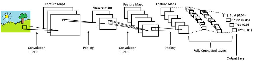
This diagram is our roadmap. Let's walk through it, step by incredible step.

Step 1: The Input Image
It all begins with our raw input: a simple image of a cartoon landscape. To the network, this is a height × width × 3 volume of pixel values. It has no concept of "sun," "tree," or "grass." It just sees numbers.

Step 2: First Convolutional Block (CONV + RELU + POOL)

• CONV: The image is first hit by a set of filters (e.g., 16 of them). These are our simplest "clue finders." The network, through training, has learned that these first-layer filters should activate for very basic patterns. One filter might learn to detect the sharp diagonal lines of the sun's rays. Another might learn to detect the vertical edge of the tree trunk. Another might activate on the color green. The output is a stack of 16 smaller "feature maps," each highlighting where its specific feature was found.

• RELU: The ReLU activation is applied to all 16 feature maps, setting any negative values to zero. This introduces non-linearity and helps the network decide which features are "on."

• POOL: A Max Pooling layer is applied. The size of each feature map is cut in half (e.g., from 24x24 to 12x12), making the representation more manageable and robust. The output is now a smaller, deeper 12 × 12 × 16 volume. This volume no longer represents pixels; it represents the locations of basic edges and color patches.

Step 3: Second Convolutional Block (CONV + RELU + POOL)
The process repeats, but now we're working with the more abstract feature maps from the previous block, not the original pixels.

• CONV: A new, second set of filters (e.g., 32 of them) is applied to the 12 × 12 × 16 input volume. These filters learn to combine the simple features from the first layer into more complex ones. A filter here might learn to activate when it sees a "vertical edge feature" next to a "green blob feature," effectively learning to recognize "tree trunk." Another filter might learn to combine several "diagonal line features" in a circular pattern to create a "sun shape" detector.

• RELU & POOL: Again, ReLU and Pooling are applied, further shrinking the dimensions (e.g., to 6 × 6) but increasing the depth (to 32). Our volume is now 6 × 6 × 32. It's a highly abstract, information-dense representation of the original image.

The Hierarchy of Features

This is the beauty of a deep CNN. The features become more complex and abstract as we go deeper into the network:

• Layer 1: Detects simple edges, corners, and color blobs.

• Layer 2: Combines edges to detect simple shapes like circles, squares, and textures.

• Deeper Layers: Combine shapes to detect object parts like eyes, noses, wheels, or leaves.

• Final Layers: Combine object parts to recognize entire objects like faces, cars, or trees.

Step 4: The Classification Head (FLATTEN + FULLY CONNECTED)

• FLATTEN: The final 6 × 6 × 32 volume is "unrolled" into one long vector. This vector is our final, comprehensive summary of all the features found in the image.

• FULLY CONNECTED: This feature vector is fed into one or more fully connected layers. This is the part of the network that performs the final reasoning. It takes the list of detected features ("sun shape found," "tree trunk found," "grass texture found") and learns how to map this combination of evidence to a final label.

• SOFTMAX: The very last layer uses a Softmax function to produce the final output: a set of probabilities for each possible class. In our example, it might correctly output Tree: 0.9.

And there you have it. The complete journey. From a meaningless grid of pixels, through a hierarchical process of feature extraction and abstraction, to a final, confident classification. It's a beautiful, powerful, and surprisingly intuitive strategy for teaching a machine how to see.

7. Going Deeper: See CNN in Action with the Vizuara AI Learning Lab!

Reading about a CNN is one thing. Seeing the filters activate and the feature maps evolve is another. To truly understand how a machine learns to see, you have to get your hands dirty and watch the magic happen.

That's why we've built the next part of our series in the Vizuara AI Learning Lab.

This isn't just another code tutorial. It's a hands-on, interactive environment where you become the architect. You will build a CNN from scratch, visualize the filters and more.

Ready to get your hands dirty? Visit the Vizuara AI Learning Lab now!

8. Conclusion

Our journey began with a simple but profound question: how can we teach a machine to see? We quickly discovered that our old tools were not up to the task. Treating an image as a simple line of pixels, as a standard feedforward network does, is an act of informational vandalism it destroys the very spatial structure that gives an image its meaning.

Then came the brilliant solution inspired by our own biology: the Convolutional Neural Network. We saw how this elegant architecture embraces the grid-like nature of images. We followed the strategy of the detective, using sliding filters (the magnifying glasses) to scan for clues (features) and create feature maps that tell us what was found and where. We saw how stacking these layers allows the network to build a hierarchical understanding of the visual world from simple edges to complex objects. Finally, we watched as all this evidence was weighed in a fully connected layer to deliver a final, confident verdict.

In essence, you now understand the complete story of how a machine learns to see. It’s not about memorizing pixels. It's about learning a process of decomposition and recognition, a dance of filters and activations that turns raw data into meaningful insight. This is the core technology that powers everything from your phone's photo gallery to self-driving cars and medical image analysis. You've decoded another fundamental pillar of modern AI.

So.. that's all for today.

Follow me on LinkedIn and Substack for more such posts and recommendations, till then happy Learning. Bye👋