
Decoding Linear Regression: How Machines Learn by Minimizing Errors
Inside the hidden mechanics of the best-fit line, cost functions, and the "downhill walk" of Gradient Descent that powers modern AI.

Table of content
Introduction: The Quest for Patterns
The Problem: Making Sense of Scattered Data
The "Best-Fit Line": Our Mathematical Crystal Ball
How Do We Measure "Best"? The Cost Function
The Strategy: Finding the Lowest Point with Gradient Descent
Deep Dive: The Math of Gradient Descent
Going Deeper: See Gradient Descent in Action with the Vizuara AI Learning Lab!
Conclusion
1. Introduction: The Quest for Patterns
Look around you. The world is not random. From the predictable cycle of the seasons to the way a coffee shop gets busier during the morning rush, our universe is built on a foundation of patterns and relationships. As humans, our brains are incredible pattern-matching machines. We intuitively understand that more hours spent studying often leads to a better grade, or that a car's price is heavily influenced by its age. We make these connections effortlessly, using them to navigate our lives and make informed decisions.
But what if we could teach a machine to do the same? What if we could give a computer a set of raw, jumbled data and empower it to find the hidden relationships within? This is the fundamental quest of machine learning: to create algorithms that can learn from data, identify underlying patterns, and use those patterns to make predictions about the future.
At the very heart of this quest lies one of the most foundational and intuitive algorithms ever conceived: Linear Regression.
Linear Regression is our first step in teaching a machine to "think" about the relationship between two or more variables. Its primary purpose is to answer a simple yet powerful question: "If I know something about Variable A, what can I predict about Variable B?"
By analyzing how changes in one variable correspond to changes in another, Linear Regression helps us gain insights, quantify relationships, and forecast future outcomes. It's the go-to method for a vast range of practical applications, from predicting a company's sales based on its advertising budget to estimating a house's price based on its square footage.
While there are several flavors of this technique, they all share the same core idea.

Simple Linear Regression: This is the most basic form, where we try to understand the relationship between just two variables, a single input and a single output. For example, predicting a student's final exam score based only on the number of hours they studied. This will be our focus for this deep dive.
Multiple Linear Regression: This is an extension where we use multiple inputs to predict a single output. For instance, predicting a car's fuel efficiency based on its engine size, weight, and horsepower.
Polynomial Regression: This is a more flexible variation that can model curved relationships in the data, not just straight lines.
In this article, we are going to pull back the curtain on Simple Linear Regression. We won't just look at what it does; We'll explore the hidden mechanics of how a machine goes from looking at a cloud of scattered data points to finding the single "best" line that can predict the future. We'll uncover the genius of cost functions and take our first steps on the "downhill walk" of Gradient Descent, a core concept that powers even the most advanced AI today.
2. The Problem: Making Sense of Scattered Data
Every machine learning journey begins with data. Not clean, perfect, pre-packaged data, but often messy, scattered, real-world data. Imagine we've been given a dataset from a college's placement cell. This dataset contains just two columns of information for a group of recent graduates: their final CGPA (Cumulative Grade Point Average) and the salary package they received (in LPA, or Lakhs Per Annum).
Our task is to build a model that can predict the salary a future student might receive, given their CGPA.
The first, most crucial step in any data-related task is always the same: visualize the data. We need to see what we're working with. So, we take the two columns of numbers and plot them on a 2D graph, with CGPA on the x-axis and the Package on the y-axis. The result is a cloud of points, known as a scatter plot.

What do we see when we look at this cloud of blue dots?
It's certainly not a perfect, straight line. For a given CGPA, say 7.0, we can see a range of different packages. This makes sense. In the real world, a salary isn't only determined by grades. It's influenced by dozens of other factors: the student's internship experience, their communication skills, the projects they built, the company they joined, and even their negotiation skills. These unmeasured, often random factors create noise in the data. We call this stochastic error.
However, even with this noise, a clear pattern emerges. There is an undeniable upward trend. As a student's CGPA increases, their salary package also tends to increase. The data isn't random; there is a relationship, a correlation, between these two variables.
This is the fundamental problem we face: we have a set of scattered data points that clearly suggest a relationship, but it's not a perfect one. How can we cut through the noise and capture the essence of this underlying trend? If this data were perfectly linear, our job would be easy. All the points would fall neatly on a single line.

If our data looked like that, we could simply draw a line that passes through every single point. We could find the exact equation of that line, and our model would be perfect. But reality is messy.
So, what's the next best thing?
Instead of finding a line that passes through every point (which is impossible here), our goal is to find a single straight line that passes as closely as possible to all the points. We need to find the line that best represents the general trend of the data. This line is our model. It's our attempt to make sense of the scattered data.
This is what Linear Regression aims to do. It's a formal method for finding this "best-fit line." The rest of this article is dedicated to understanding exactly what "best" means, and how we can mathematically find the one line, out of an infinite number of possibilities, that truly is the best fit.
3. The "Best-Fit Line": Our Mathematical Crystal Ball
We've set our sights on a clear goal: to draw a single straight line that best captures the underlying trend in our scattered CGPA vs. Package data. This line will act as our predictive model. Once we have it, we can use it to estimate the package for any new CGPA. It becomes our mathematical crystal ball.
But what is a line, mathematically? From high school algebra, we know that any straight line on a 2D graph can be described by a simple and elegant equation:
y = m * x + b
This equation is the engine of our entire model. Let's break down what each part means in the context of our specific problem:
y: This is the dependent variable, the value we are trying to predict. In our case, y is the Package.
x: This is the independent variable, the input we use to make our prediction. For us, x is the CGPA.
m: This is the slope of the line. It tells us how steep the line is. The slope quantifies the relationship between x and y. It answers the question, "For every one-unit increase in CGPA, how much does the Package change?" A positive slope means the package increases as CGPA increases.
b: This is the y-intercept. It's the value of y when x is zero. It tells us where the line crosses the vertical y-axis.
These two values, m and b, are the parameters of our model. If we can find the perfect values for m and b, we can define the perfect line. The entire challenge of Linear Regression boils down to finding the optimal m and b for our specific dataset.
But this brings us back to our core problem. Our data is scattered, not perfectly linear. No matter what line we draw, it's not going to pass through every single data point. This means our model will never be perfect. For any given student's actual CGPA, our line will predict a package, but that prediction will likely be slightly different from the package that student actually received
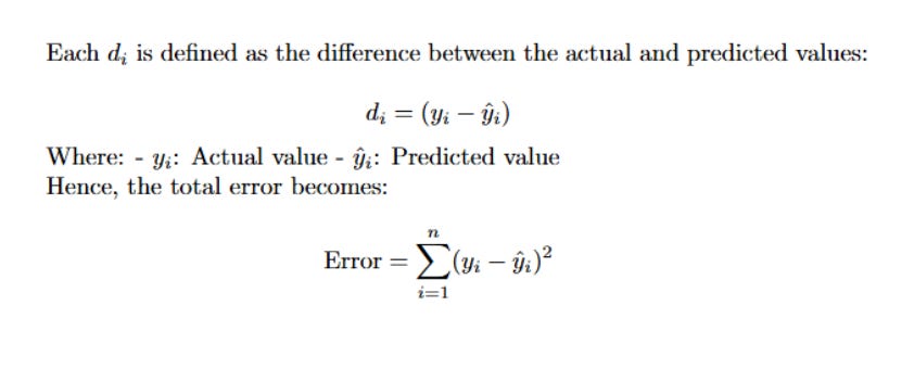
This difference between the actual value and the predicted value is the error, sometimes called the residual.
Let's visualize this. For every data point in our plot, there is a vertical distance between the blue dot (the actual data) and our red best-fit line (the model's prediction).

In this diagram:
The Actual Data (yi) is represented by the blue dots. This is the real-world package a student received.
The Best-Fit Line (ŷi) represents our model's predictions. This is the package our line thinks a student should have received based on their CGPA.
The Error (di) is the dashed grey line, the vertical distance between the actual value and the predicted value for a single student.
Our best-fit line will have some error for almost every single data point. Some points will be above the line, and some will be below it.
This leads us to the most important question in Linear Regression: If every possible line has some error, how do we define which line is "best"? The answer is simple and intuitive: The best line is the one that has the least amount of total error.
Our quest has now become more specific. We aren't just looking for a line; we are looking for the one unique line the one set of m and b that minimizes the total error across all of our data points. But how do we calculate this "total error"? That's the next piece of the puzzle.
4. How Do We Measure "Best"? The Cost Function
We've established a clear objective: find the line with the least amount of total error. This seems straightforward enough. For each of our n data points, we have an error, d. A tempting first thought might be to simply add up all these individual errors:
Total Error = d₁ + d₂ + d₃ + ... + dₙ
However, this simple approach has a critical flaw. Looking at our diagram, some data points are above the line, and some are below it.
For points above the line, the error (yi - ŷi) will be a positive number.
For points below the line, the error (yi - ŷi) will be a negative number.
If we just add them up, the positive and negative errors will start cancelling each other out. We could end up with a line that has huge errors but a total sum close to zero, which would trick us into thinking it's a good fit. We need a way to treat all errors as positive magnitudes of "wrongness."
There are two common ways to solve this:
Take the absolute value of each error: |di|.
Square each error: di².
While using the absolute value works, the machine learning community overwhelmingly prefers squaring the error. This method has two wonderful properties:
It makes all errors positive: Squaring any number, positive or negative, results in a positive number.
It penalizes larger errors more: An error of 2, when squared, becomes 4. But an error of 10, when squared, becomes 100. This means the model will be highly motivated to fix its biggest mistakes, as they contribute much more to the total error.
So, our new formula for total error becomes the Sum of Squared Errors (SSE):
E = d₁² + d₂² + d₃² + ... + dₙ²
We can write this more compactly using summation notation:

Since we know that each error di is the difference between the actual value yi and the predicted value ŷi, we can substitute that into our equation:
Error = Σ (yi - ŷi)²
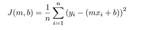
We're almost there. This gives us the total squared error. To make the number more manageable and independent of the number of data points in our dataset, we typically take the average of these squared errors. This final, averaged value is our official Cost Function. In the context of Linear Regression, it's called the Mean Squared Error (MSE).
Cost Function J(m, b) = (1/n) * Σ (yi - ŷi)²
Let's break down this final, crucial formula:
J(m, b): We call our Cost Function J, and we write it as a function of m and b. This is a critical reminder that the cost depends entirely on the line we choose that is, on the specific values of the slope m and intercept b that define the line. Change m or b, and the line changes, the predictions ŷi change, and therefore the total error J changes.
(1/n): This is just "one over the number of data points," which is how we get the mean (or average).
Σ (yi - ŷi)²: This is the "sum of squared errors" we just derived.
We have finally arrived at a precise, mathematical definition of "best." The best-fit line is no longer a vague concept. The best-fit line is the one defined by the specific values of m and b that make the value of our Cost Function, J(m, b), as small as humanly (or mechanically) possible.
Our entire complex problem has been distilled into a single, clear mission: find the minimum value of J(m, b). The algorithm that helps us do this is one of the most famous and important in all of machine learning: Gradient Descent.
5. The Strategy: Finding the Lowest Point with Gradient Descent
So, our mission is clear: find the perfect duo of m and b that results in the lowest possible value for our Mean Squared Error cost function, J(m, b).
But how do we do that? We could try to plug in millions of different values for m and b and see which combination gives the lowest error. This "brute force" approach would be incredibly inefficient and would likely never find the perfect minimum. We need a smarter, more elegant strategy.
This is where we introduce one of the most fundamental and powerful optimization algorithms in all of machine learning: Gradient Descent.
To understand the intuition behind Gradient Descent, let's use an analogy. Imagine our cost function, J(m, b), not as an equation, but as a physical landscape. Since the cost J depends on two variables, m and b, we can visualize this landscape as a 3D surface, a range of hills and valleys.

In this 3D landscape:
The two horizontal planes represent all possible values for our parameters, m and b.
The vertical height at any point represents the Cost (J) for that specific combination of m and b.
The high peaks of the hills are the combinations of m and b that produce a terrible-fitting line with a very high error.
The low points, the bottoms of the valleys, are the combinations of m and b that produce a great-fitting line with a very low error.
Our goal is to find the absolute lowest point in this entire landscape. That lowest point is the global minimum. the set of m and b that gives us our true best-fit line.
So, how do we find this lowest point? We walk downhill.
This is the beautiful, simple idea behind Gradient Descent. The algorithm works like this:
Start Somewhere Random: We begin by dropping a ball at a random starting point on this 3D surface. This is equivalent to initializing our m and b with random values.
Look Around and Find the Steepest Downhill Direction: From our current position, we need to figure out which direction is the fastest way down. In mathematical terms, we need to find the direction of the steepest descent. This is where the "gradient" comes in. The gradient is a vector of partial derivatives that always points in the direction of the steepest ascent (the fastest way uphill). Therefore, the fastest way downhill is simply the opposite direction of the gradient.
Take a Small Step: We take a small step in that negative-gradient (downhill) direction. This moves us to a new position on the landscape with a slightly lower error.
Repeat: We are now at a new point. We repeat the process: look around again, find the new steepest downhill direction from this new spot, and take another small step.
We repeat this process look, step, look, step over and over again. With each step, we move further down into the valley. Eventually, we will reach the bottom, where the ground is flat. At this point, the gradient will be zero (there's no "uphill" direction), so we stop taking steps. We have converged at the minimum. The m and b coordinates of this final resting place are the optimal parameters for our best-fit line.
This "downhill walk" is the essence of Gradient Descent. But two questions remain:
How, exactly, do we calculate the "gradient" at each step?
How big should our "steps" be?
Answering these questions requires us to dive into the math, which is exactly what we'll do next.
6. Deep Dive: The Math of Gradient Descent
We've built the intuition: Gradient Descent is an iterative process of "walking downhill" on our cost function landscape until we find the lowest point. The two magic ingredients we need are the direction of the walk and the size of our steps.
The direction is determined by the negative gradient of the cost function, J(m, b).
The size of the steps is determined by a parameter we choose called the Learning Rate (α).
Our entire algorithm will be based on these two simple update rules, which we apply over and over again:

Our task now is to find those gradients. The gradient is a vector of partial derivatives.
We need to find two partial derivatives:
The partial derivative of the Cost Function J with respect to m (written as ∂J/∂m). This tells us how the cost changes as we slightly change the slope m.
The partial derivative of the Cost Function J with respect to b (written as ∂J/∂b). This tells us how the cost changes as we slightly change the intercept b.
Let's tackle these one at a time.
Step 1: Setting up the Equation
First, let's write out our full Cost Function again. Remember that ŷi (the prediction) is just our line's equation, m*xi + b. Let's substitute that in:

This is the equation we need to differentiate. It looks intimidating, but we'll break it down using a fundamental rule from calculus: the Chain Rule. The Chain Rule helps us differentiate composite functions, functions that are nested inside other functions.
Step 2: Calculating the Gradient for the Slope (∂J/∂m)
We want to find ∂J/∂m. Let's focus on the part of the equation that actually contains m. For a single data point i, the squared error is (yi - (m*xi + b))².
To make the Chain Rule clearer, let's define an intermediate variable, E, as the expression inside the square:

So the squared error is just E².
The Chain Rule tells us that the derivative of E² with respect to m is:

Now we just need to solve the two parts of this:
2 * E: This is simple. We just substitute E back in: 2 * (yi - (m*xi + b)).
∂E/∂m: This means we need to find the derivative of E with respect to m. Let's look at E = yi - m*xi - b.
The derivative of yi with respect to m is 0 (because yi is a constant value that doesn't depend on m).
The derivative of -m*xi with respect to m is -xi (because xi is treated as a constant coefficient of m).
The derivative of -b with respect to m is 0 (because b is a constant with respect to m).
So, ∂E/∂m = 0 - xi - 0 = -xi.
Now, let's put it all back together for a single data point:

This is the derivative of the squared error for just one data point. Our full cost function J(m, b) sums this up over all n data points and takes the average. So, we apply the sum and the (1/n) factor:

Let's clean that up a bit by moving the constants -1 and 2 outside the summation:

And since (m*xi + b) is just our prediction ŷi, we can write it even more cleanly:

That's it! We've done it. We have derived the first half of our gradient. This formula gives us a precise value that tells us, at our current position (m, b), which direction is "uphill" for the slope m. To go downhill, we will move in the opposite direction.
Next, we'll do the same for b.
Step 3: Calculating the Gradient for the Intercept (∂J/∂b)
Now we need to find the second part of our gradient: the partial derivative of the Cost Function J with respect to the intercept b (written as ∂J/∂b).
We start with the same full Cost Function equation:
Again, we'll use the Chain Rule. We can use the same intermediate variable E that we defined before, because the overall structure of the function is the same.

The squared error is E².
The Chain Rule tells us that the derivative of E² with respect to b is:

Let's solve the two parts of this expression for b:
2 * E: This part is identical to before. It's 2 * (yi - (m*xi + b)).
∂E/∂b: This is the new part. We need to find the derivative of E with respect to b. Let's look at E = yi - m*xi - b.
The derivative of yi with respect to b is 0 (it's a constant).
The derivative of -m*xi with respect to b is 0 (it's also treated as a constant).
The derivative of -b with respect to b is -1.
So, ∂E/∂b = 0 - 0 - 1 = -1.
Now, we combine these pieces for a single data point's squared error:

This is the derivative for just one data point. To get the final gradient for our cost function J(m, b), we sum this across all n data points and multiply by (1/n) to get the average:

Let's clean this up by moving the constants -1 and 2 out of the summation:

And finally, since (m*xi + b) is our prediction ŷi, we can write the formula in its cleanest form:
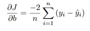
And there we have it! This is the second half of our gradient. This formula tells us which direction is "uphill" for the intercept b.
Step 4: The Final Update Rules and the Learning Rate
We have successfully derived both parts of the gradient. Now we can write out the complete, final update rules for one step of Gradient Descent:

The Gradient Descent algorithm then simply involves initializing m and b to some random values (often 0) and then repeatedly applying the following updates:

The Learning Rate (α) is a small positive number (e.g., 0.01, 0.001) that we choose ourselves. It's a "hyperparameter" of our model. The learning rate is crucial:
If α is too small: We will take tiny, tiny steps downhill. We will eventually reach the bottom, but it might take a very long time and a lot of computational power.
If α is too large: We might take steps that are too big. We could overshoot the bottom of the valley and end up on the other side, potentially with an even higher error than before. It's like trying to walk down a hill by taking giant leaps; you might miss the bottom entirely.
Finding a good learning rate is a key part of training a machine learning model.
We repeat this process of calculating the gradients and updating m and b for a set number of iterations (or "epochs"), or until the cost J stops decreasing significantly. With each iteration, our line y = mx + b gets closer and closer to the true best-fit line, and our model "learns" the relationship hidden in our data.
7. Going Deeper: Perform the Math with the Vizuara AI Learning Lab!
We've journeyed through a lot of theory from the simple equation of a line to the calculus of partial derivatives. But to truly internalize how this works, reading isn't enough. You have to do the math.
That's why we've built a different kind of interactive lab. This isn't a simulation you just watch. This is a hands-on environment where you become the Gradient Descent algorithm. You will step through the process, performing the crucial calculations yourself to see how the numbers actually crunch and flow.
Ready to get your hands dirty? Visit the Vizuara AI Learning Lab now!
8. Conclusion
We started our journey with a simple question and a cloud of scattered data: "Can we predict a student's salary based on their CGPA?" This led us down a path to uncover one of the most fundamental algorithms in all of machine learning.
First, we saw that the problem wasn't about finding a perfect line, but a "best-fit line" our mathematical crystal ball for making predictions.
Then, we gave a precise definition to the word "best." The best line, we discovered, is the one that minimizes the total error. We quantified this error using a Cost Function, the Mean Squared Error, which measures the average squared distance between our model's predictions and the actual data.
Our mission became clear: find the values of m and b that result in the lowest possible cost.
Finally, we unveiled the strategy to achieve this: Gradient Descent. We learned the beautiful intuition of "walking downhill" on a 3D error landscape. We didn't just accept it as magic; we dove into the calculus and derived the exact formulas the partial derivatives that tell our algorithm which way is "down" at every single step.
In essence, you now understand the complete story of how a machine can learn from data. It starts with a model (y = mx + b), measures its performance with a cost function, and then iteratively improves that model using an optimization algorithm like Gradient Descent. This core loop of Model -> Cost -> Optimization is not just for linear regression; it is the beating heart of nearly all of modern AI, from image classifiers to the most advanced large language models.
You've decoded the fundamentals. The rest of machine learning is just building on these powerful ideas.
So.. that's all for today.
Follow me on LinkedIn and Substack for more such posts and recommendations, till then happy Learning. Bye👋