
Decoding Multi-Head Latent Attention (Part 1): The KV Cache Memory Bottleneck, Solved.
Discover why the KV Cache is the biggest bottleneck in LLM inference, how MQA and GQA tried to fix it, and how DeepSeek's Latent Attention masterfully solves the problem by learning to compress memory

Table of content
Introduction: The Unseen Challenge of LLM Memory
The Problem: The Ever-Growing KV Cache and Its Memory Wall
Prior Attempts: MQA, GQA, and Their Compromises
The Solution: Multi-Head Latent Attention, The Master Sketch Artist
Deep Dive: How Latent Attention Compresses and Reconstructs
The Payoff: Unleashing Lightning-Fast Inference
Going Deeper: Experience Latent Attention in the Vizuara AI Lab!
Conclusion
References
1. Introduction: The Unseen Challenge of LLM Memory
Think about conversing with a Large Language Model (LLM) like DeepSeek-V2. You ask it a complex question, perhaps a multi-turn dialogue, or you feed it a lengthy document for summarization. It responds with startling coherence, understanding context, and generating text that feels remarkably human-like. It's almost as if it "remembers" everything you've said, every detail from the document, perfectly aligning its responses to the ongoing conversation.

This incredible ability to understand and generate long sequences of text is what has pushed the boundaries of Artificial Intelligence, hinting at a future we once only dreamed of. From crafting creative stories to assisting with complex coding tasks, LLMs have fundamentally changed how we interact with machines.
But here's a secret, a subtle challenge hidden beneath the surface of their impressive capabilities: how do these colossal models actually hold onto all that information during a conversation? How do they remember the beginning of a 100,000-word document when they're generating the last sentence?
This isn't just a theoretical curiosity. It's a critical, practical challenge that impacts how fast, how economically, and how effectively these powerful models can operate in the real world. While the raw intelligence of LLMs has soared, their memory management has quietly become a significant bottleneck.
In our previous blogs, we explored how neural networks learn from data: from predicting continuous values with lines, to classifying outcomes with probabilities, to understanding word meaning, and even gaining a basic "memory" for sequences with RNNs. But handling the sheer scale of conversation history in modern LLMs presents a unique, unseen challenge – a memory problem of colossal proportions.
Today, we're going to pull back the curtain on this unseen challenge. We'll explore the ingenious architectural innovation that DeepSeek has pioneered to tackle this head-on: Multi-Head Latent Attention (MLA). It's a clever twist on the attention mechanism that drastically reduces the memory footprint, enabling LLMs to remember more, generate faster, and run more economically than ever before.
Section 2: The Problem: The Ever-Growing KV Cache and Its Memory Wall
In our previous explorations of RNNs and attention, we touched upon how models process sequential data. Now, let's zoom in on the most common architecture for Large Language Models (LLMs): the Transformer. At its heart, the Transformer uses an ingenious mechanism called Multi-Head Attention (MHA) to understand context. Remember the core idea: Queries (Q) look for relevant information in Keys (K), and then extract that information from Values (V).
For tasks like text generation (what LLMs do best), models work in an autoregressive manner. This means they generate text token by token, one word after another, based on all the words that came before it. Think of it like someone writing a very long story, sentence by sentence. To write the next word, they need to keep the entire story written so far in mind.
In the world of Transformers, this "keeping the entire story in mind" translates to a massive computational burden. To generate each new token, the model needs to calculate attention not just with the current token, but with all the preceding tokens in the sequence. Without a clever optimization, for every new token, the model would have to re-compute the Key and Value vectors for the entire historical context from scratch. This would be incredibly inefficient, making long-sequence generation practically impossible.
Imagine reading the same 100-page book from the beginning every time you want to write down the next word of a summary. It's ludicrous!
This is where the Key-Value (KV) Cache comes to the rescue.
The KV Cache is a brilliant optimization designed to speed up autoregressive decoding. Instead of re-computing the Keys and Values for all previous tokens at each step, the Transformer simply computes them once for each token and then stores (caches) them in memory. As the model generates a new token, it adds its newly computed Key and Value to this cache. Then, for the next token, it reuses the Keys and Values already in the cache, only computing the new Query vector.
This dramatically speeds up inference by avoiding redundant computations. It's like our diligent author keeping a running "summary sheet" of the story so far. Every time they write a new word, they just add it to the summary sheet, instead of re-reading the whole book. This allows LLMs to process incredibly long contexts, often hundreds of thousands of tokens.
However, the speedup achieved by the KV Cache comes at a significant cost: memory.
The brilliance of the KV Cache quickly runs into a harsh reality when we scale up to modern Large Language Models: memory consumption becomes astronomically high, creating a severe bottleneck for inference efficiency.
Let's break down why this happens. The size of the KV Cache (the total number of elements it needs to store) scales with several factors:
Batch Size (B): How many different input sequences (e.g., conversations with different users) the model is processing simultaneously.
Sequence Length (L): The total length of the conversation history or input document. This is the accumulated tokens generated so far.
Hidden Dimension (d): The size of the vector representation for each token.
Number of Attention Heads (nh): How many different "perspectives" the attention mechanism uses.
Number of Layers (N_layers): The depth of the Transformer model (each layer has its own attention block and thus its own KV cache).
For every token in every sequence in every batch, we need to store two vectors (Key and Value) for each attention head in each Transformer layer. So, the total KV Cache size per layer is roughly:
2 × L × d × nh (elements)
And for the entire model, it's N_layers × (2 × L × d × nh).
Consider DeepSeek-V2, for instance. It boasts a context length of 128,000 tokens. Imagine trying to hold a KV Cache for that many tokens! A single full-sized KV Cache for a large LLM can easily consume tens to hundreds of gigabytes of GPU memory.
This immense memory footprint leads to critical limitations:
Limited Batch Size: GPUs have finite memory. If the KV Cache for one long sequence is already huge, you can only fit a very small number of parallel sequences (batch size) onto the GPU. A smaller batch size directly translates to lower throughput (fewer tokens generated per second), making the LLM expensive and slow to use in real-time applications.
Limited Context Length: Even if you process one sequence at a time (batch size 1), there's a hard limit to how long the conversation can be before the KV Cache overflows the GPU's memory. This restricts the practical applications of LLMs for very long documents or extended dialogues.
High Inference Costs: More memory means more expensive GPUs, and lower throughput means more GPUs needed to serve the same number of users, driving up operational costs.
This is the very real, very painful "memory wall" that has plagued LLMs, despite their computational prowess. It's not about the speed of computation anymore; it's about the speed and quantity of data that can be stored and accessed during inference.
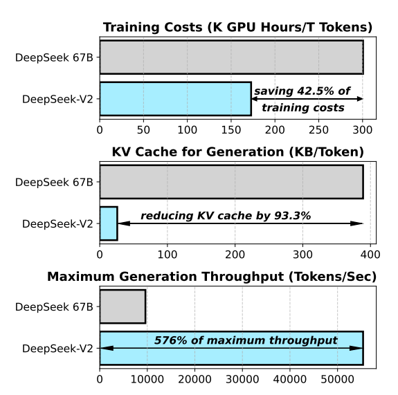
As you can see in that graph, DeepSeek-V2 dramatically reduces the KV Cache size(by 93.3%) compared to its predecessor, DeepSeek 67B. This isn't just a minor improvement; it's a monumental achievement that unlocks truly efficient large-scale LLM deployment.
But how did they achieve this? How do you shrink a core component of the Transformer without breaking its remarkable performance? This brings us to the ingenious solutions that attempt to tackle this memory monster.
3. Prior Attempts: MQA, GQA, and Their Compromises
So, the engineering world faced a classic trade-off: use a full KV Cache for maximum model performance but suffer from a massive memory footprint, or find a way to shrink it and risk hurting the model's intelligence. This challenge gave birth to some clever, but ultimately compromised, solutions. Let's look at the two most famous ones: Multi-Query Attention and Grouped-Query Attention.
a. Multi-Query Attention (MQA): Sharing All Keys, For Better or Worse
The first radical idea was Multi-Query Attention (MQA). The logic was simple and brutal: "What if we just... didn't store all those different Key and Value heads?"
In MQA, while you still have multiple Query heads (let's say, 32 of them), you force all of them to share a single Key head and a single Value head.
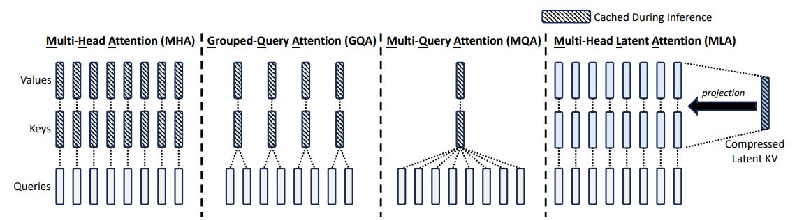
Look at the MQA column in that diagram. It's a stark contrast to the MHA column. All those independent Key and Value streams have been collapsed into one.
The Good: The memory savings are enormous. Instead of storing, say, 32 sets of Keys and Values in the cache, you're only storing one. This drastically shrinks the KV Cache, allowing for much larger batch sizes and longer context windows on the same hardware.
The Bad: This efficiency comes at a steep price. Forcing every query head, each trying to look for different information, to use the same Key and Value "summary" is a major compromise. It's like giving our team of 32 detectives only one shared notepad. It leads to a noticeable drop in model quality and performance. The model becomes less nuanced and less capable.
b. Grouped-Query Attention (GQA): A Middle Ground
MQA was too extreme. So, the community developed a compromise: Grouped-Query Attention (GQA).
GQA is the logical middle ground between the "one-for-all" of MQA and the "one-for-each" of MHA. It splits the Query heads into several groups and assigns a single shared Key and Value head per group.
For example, our 32 query heads might be split into 4 groups of 8. Each group of 8 queries would then share one K/V head.
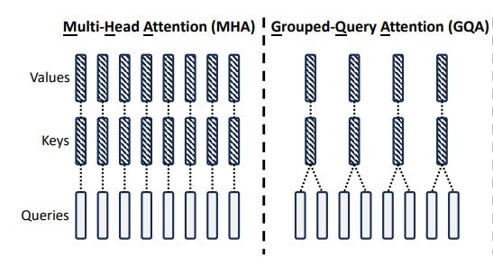
As you can see in the GQA column, it's a perfect blend of the other two ideas.
The Good: GQA offers a much better balance. It achieves significant memory savings over MHA while suffering much less of a performance hit than MQA. It quickly became the go-to standard for many popular open-source models that needed to be efficient without sacrificing too much quality.
The Unavoidable Trade-off
Both MQA and GQA made great strides, but they couldn't escape the fundamental trade-off. They both reduced the "expressiveness" of the model in exchange for a smaller memory footprint. They were clever workarounds, but they felt like compromises, not true solutions.
The holy grail remained elusive: Is it possible to shrink the KV Cache dramatically while not just maintaining, but improving upon the performance of standard Multi-Head Attention?
The answer, as DeepSeek discovered, is yes. And it requires a completely different way of thinking about the problem.
4. The Solution: Multi-Head Latent Attention — The Master Sketch Artist
So, we've seen the problem: the KV Cache is a memory monster. And we've seen the prior attempts: MQA and GQA, clever compromises that sacrificed model quality for a smaller memory footprint. This is where the team at DeepSeek stepped back and asked a fundamentally different question. Instead of asking, "How can we share or reduce the number of Key and Value heads?", they asked, "Why are we storing the full, high-dimensional Key and Value vectors at all?"
This question is the key that unlocks the genius of Multi-Head Latent Attention (MLA).
The core insight is this: the high-dimensional Key and Value vectors, while necessary for the attention calculation, might contain a lot of redundant information. What if the true "essence" of what the model needs to remember from a past token could be captured in a much, much smaller space?
This is where our master analogy comes into play.
Our Analogy: The Master Sketch Artist
Imagine our LLM is a detective investigating a very long and complex case (the input sequence).
Standard MHA (with KV Cache): The detective, after reading each witness statement (each token), makes a perfect, life-sized, full-color oil painting of the scene (the Key and Value vectors). They store this giant painting in a warehouse (the KV Cache). To understand a new clue, they have to pull out all the previous giant paintings to get the full context. The warehouse gets full very quickly. This is the memory bottleneck.
MQA/GQA: The detective decides to save space by just taking a few low-resolution photographs instead of full paintings. It saves space, but crucial details are lost. This is the quality degradation we saw.
Multi-Head Latent Attention (MLA): The detective hires a Master Sketch Artist. This artist is a genius at capturing the absolute essence of a scene. After the detective reads a witness statement, the artist doesn't create a giant oil painting. Instead, they create a small, information-dense, black-and-white latent sketch (the latent vector). This sketch is tiny, but it contains all the critical information: the lines, the shapes, the mood. The detective stores these small sketches in their notepad (the new, tiny KV Cache).
Now, when a new clue comes in, the detective doesn't need the original paintings. They simply show the relevant past sketches to the artist. The artist, with their incredible skill, can look at a small sketch and instantly re-create a rich, detailed, full-color mental image (the reconstructed Key and Value vectors) of that past event, just for the moment it's needed for the attention calculation.
This is the beautiful, core idea of MLA.
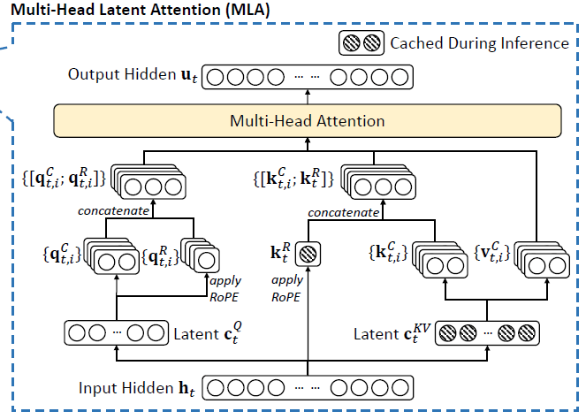
This diagram shows our sketch artist at work. The process isn't about sharing or grouping; it's about Compress -> Store -> Reconstruct.
Compress (Creating the Sketch): The model takes the full input for a token (h_t) and uses a special learned matrix to compress it into a tiny latent vector (c_KV).
Store (Saving the Sketch): This tiny c_KV is the only thing that gets saved in the Key-Value cache for that token.
Reconstruct (Re-creating the Painting): When it's time to perform attention, the model retrieves the stored latent sketches (c_KV) and uses other learned matrices to instantly "up-project" them back into the full-sized Key and Value vectors needed for the calculation.
This simple, elegant idea completely reframes the problem. We are no longer fighting with memory by reducing the number of K/V heads. We are tackling the problem at its source by reducing the size of the information we store for each head.
5. Deep Dive: How Latent Attention Compresses and Reconstructs
The Setup: Our Input and Weight Matrices
Everything begins with two things: our input data and the network's learned parameters (the weights).
The Input Hidden State (h_t): This is the vector representing the current token after it has passed through the lower layers of the Transformer. For our example, let's say it's a simple vector of 8 dimensions.
h_t (1x8 vector)The Weight Matrices (The Learned "Skills"): The network has five key weight matrices that it has learned during its training phase. These are the tools our sketch artist uses.
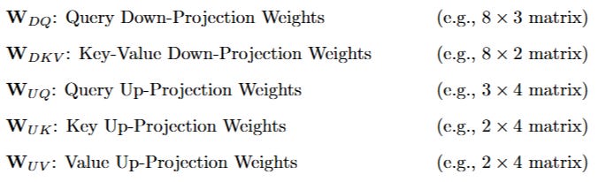
Our mission is to trace h_t as it interacts with these matrices to produce the final q, k, and v vectors for the attention calculation.
Step 1: The Fork in the Road - Compressing the Query and KV
The first thing the network does is send the input hidden state h_t down two parallel paths simultaneously.
Path A: Compressing the Query
The network calculates the latent query vector (c_q). This is done by multiplying the input h_t by the query down-projection matrix W_DQ.
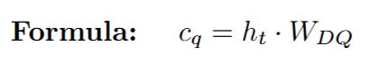
Let's look at the dimensions to understand the compression:
The matrix multiplication effectively compresses the 8-dimensional input into a much smaller 3-dimensional latent representation for the query. This c_q is a temporary variable used to reconstruct the final query.
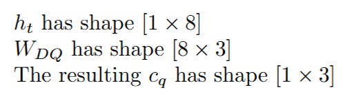
Path B: Compressing the Key and Value
Simultaneously, the network calculates the shared latent KV vector (c_KV). This is the vector that will actually be stored in the cache. It's created by multiplying the same input h_t by the KV down-projection matrix W_DKV.
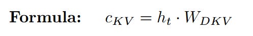
Again, let's check the dimensions:
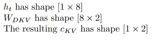
Notice the aggressive compression here! The 8-dimensional input has been squeezed into a tiny 2-dimensional vector. This is our "latent sketch." This incredibly small vector is what's stored in the KV Cache, saving an immense amount of memory compared to storing the full-dimensional Key and Value vectors.
At this point, the compression phase is complete. We have successfully created our low-dimensional sketches.
Our network has successfully performed the compression. It holds two small, information-dense latent vectors:
c_q: The latent query (shape [1 x 3]).
c_KV: The latent Key-Value sketch (shape [1 x 2]), which is the vector we would store in our cache.
These vectors are too small to be used in the standard attention mechanism, which expects q, k, and v to have the same dimension (the head dimension, d_h). The next phase is to reconstruct these full-sized vectors from our compressed sketches. This is achieved through another set of learned weight matrices in a process called up-projection.
Step 2: Reconstructing the Query, Key, and Value
Reconstructing the Query (q)
The network takes the latent query c_q and multiplies it by the query up-projection matrix W_UQ to restore it to the full head dimension.
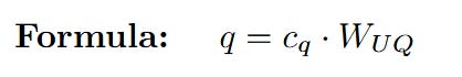
Let's trace the dimensions:
The 3-dimensional latent query is now projected back into a full 4-dimensional query vector, ready for the attention calculation.
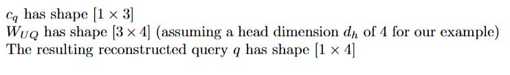
Reconstructing the Key (k) and Value (v) from the Shared Sketch
This is where the true elegance of MLA shines. The network uses the single, shared latent KV vector c_KV to reconstruct both the Key and the Value, using two separate up-projection matrices.
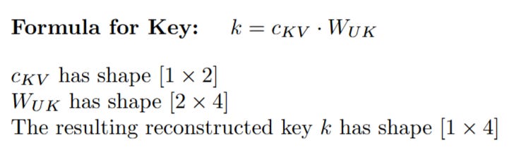
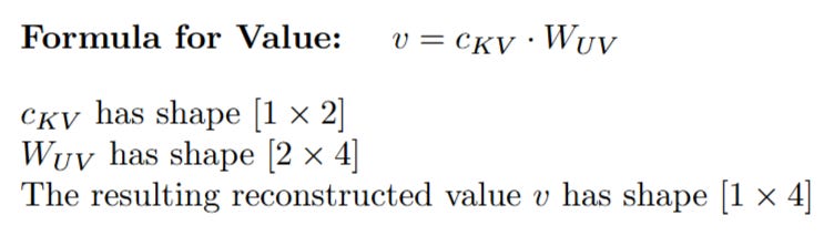
Notice how the tiny 2-dimensional sketch c_KV was able to generate both a 4-dimensional Key and a 4-dimensional Value. Because W_UK and W_UV have different learned weights, they can interpret the compressed information in c_KV differently, extracting the necessary aspects for "what I have" (the Key) and "what I will give" (the Value).
Step 3: The Final Attention - Business as Usual
Now that we have our fully reconstructed q, k, and v vectors, all of the same dimension (d_h = 4), the rest of the process is identical to the standard Multi-Head Attention we know and love.
The model calculates the dot product between the query q and the transpose of the key k, scales it, applies a Softmax function to get the attention weights, and then multiplies those weights by the value vector v to get the final output.
This entire, elegant dance of matrices compressing the input into tiny latent sketches and then reconstructing them just in time for the attention calculation—is the core mechanism of Multi-Head Latent Attention. It solves the KV Cache memory problem at its source, not by compromising on the number of attention heads, but by being smarter about what information it chooses to remember.
6. The Payoff: Unleashing Lightning-Fast Inference
We've journeyed through the intricate mathematics of low-rank projections and seen how MLA cleverly compresses and reconstructs information. While the process is elegant, the true reward the reason this architecture is so revolutionary lies in its staggering real-world impact on performance. By solving the KV Cache memory wall, MLA unlocks a new level of efficiency for Large Language Models.
Let's quantify this payoff.
a. KV Cache Reduction: From a Flood to a Trickle
The primary goal of MLA was to shrink the memory footprint of the KV Cache, and on this front, the results are nothing short of breathtaking.
Let's recall the problem: in standard Multi-Head Attention (MHA), the cache size per token is 2 × nh × dh (where nh is the number of heads and dh is the dimension per head). For a large model, this can be enormous.
In MLA, we are no longer storing the full Key and Value vectors. We are only storing the tiny, shared latent vector, c_KV. The size of this vector is dc.
The results from the DeepSeek team speak for themselves.
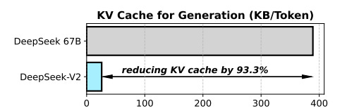
As shown in their research, compared to their powerful 67B dense model, DeepSeek-V2 with MLA reduces the KV cache size by an incredible 93.3%!
This isn't just an incremental improvement; it's a fundamental change in the economics of inference. What was once a memory-chugging giant becomes a lean, efficient machine. This massive reduction in memory usage has two direct consequences:
Longer Context Windows: Models can handle vastly longer sequences of text before running out of GPU memory.
Larger Batch Sizes: More sequences can be processed in parallel on the same hardware, dramatically increasing server capacity.
b. Boosting Generation Throughput: Speed Beyond Expectations
Reduced memory is fantastic, but does it translate to raw speed? Absolutely. Throughput, measured in tokens generated per second, is the ultimate metric for inference efficiency. By allowing for larger batch sizes, MLA directly leads to a massive boost in throughput.
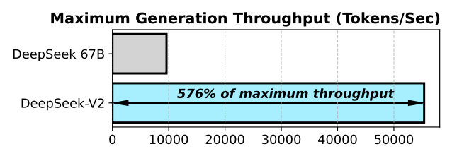
The data is clear. Benefiting from the tiny KV cache and other optimizations, DeepSeek-V2 achieves a generation throughput 5.76 times higher than its dense MHA-based predecessor.
This is the ultimate payoff. MLA doesn't just manage the memory problem; it crushes it, unlocking a level of performance that makes large-scale, long-context LLM applications more feasible and cost-effective than ever before. It proves that you don't have to choose between model quality and inference efficiency. With a clever enough architecture, you can have both.
But what's even more exciting is that you can experience this process yourself.
7. Going Deeper: Experience MLA in the Vizuara AI Lab!
Theory and diagrams are one thing, but to truly internalize how a high-dimensional vector can be squashed into a tiny sketch and then brought back to life, you need to perform the calculations yourself. You need to see the numbers crunch and flow.
That's why we've built the next part of our advanced architecture series in the Vizuara AI Learning Lab. This isn't a passive video or a block of code to copy. It's a hands-on, interactive environment where you become the computational engine of the MLA layer. You will:
Manually perform the matrix multiplications for both the down-projection and up-projection steps.
Create the latent vectors c_q and c_KV from the hidden state, and see the dimensionality reduction with your own eyes.
Reconstruct the full q, k, and v vectors and validate your results against the expected output.
Reading is knowledge. Calculating is understanding. Are you ready to master the mechanics of modern LLM efficiency?
8. Conclusion
Our journey began with a critical, yet often overlooked, challenge in the world of Large Language Models: the memory wall. We saw how the very mechanism that allows LLMs to "remember" long contexts, the KV Cache becomes a massive bottleneck, limiting speed, scalability, and economic feasibility.
We explored the early attempts to solve this, MQA and GQA, which made a difficult trade-off between memory and model performance. Then came the paradigm shift with Multi-Head Latent Attention. Instead of compromising, MLA reframed the problem entirely. By using the elegant mathematics of low-rank projections, it showed us that we don't need to store the entire memory; we only need to store a compressed, latent "sketch."
We walked through this process step-by-step, seeing how the network acts as a "Master Sketch Artist," compressing high-dimensional information into tiny latent vectors and then reconstructing it on-demand. The payoff is a revolutionary leap in efficiency a 93% reduction in cache size and a nearly 6x increase in generation throughput.
However, our story isn't quite finished. We've mastered the core compression mechanism in its purest form. But there's a crucial piece we've intentionally left out: positional information. How does the model know the order of the tokens when we're doing all this compression? Directly applying standard techniques like RoPE would break the beautiful efficiency we've just achieved.
Solving that puzzle requires another layer of ingenuity. And that will be the subject of Part 2 of our series, where we will explore the "Decoupled RoPE" trick that makes MLA truly complete.
9. References
This article is a conceptual deep dive inspired by the groundbreaking work of researchers and engineers in the AI community. For those wishing to explore the source material and related concepts further, we highly recommend the following papers and resources:
[1] DeepSeek-AI. (2024). DeepSeek-V2: A Strong, Economical, and Efficient Mixture-of-Experts Language Model. arXiv:2405.04434
[2] Liu, A., Feng, B., et al. (2024). Deepseek-v3 technical report. arXiv:2412.19437
[3] Vaswani, A., Shazeer, N., et al. (2017). Attention Is All You Need. arXiv:1706.03762
[4] Shazeer, N. (2019). Fast Transformer Decoding: One Write-Head is All You Need. arXiv:1911.02150
[5] Ainslie, J., Lee-Thorp, J., et al. (2023). GQA: Training Generalized Multi-Query Transformer Models from Multi-Head Checkpoints. arXiv:2305.13245
Stay Connected
So.. that's all for today.
Follow me on LinkedIn and Substack for more such posts and recommendations, till then happy Learning. Bye👋