Decoding Multi-Head Latent Attention (Part 2): Solving the RoPE Paradox

In Part 1, we solved the memory wall with latent compression. Now, discover how standard RoPE breaks this efficiency and why DeepSeek's "Decoupled RoPE" is the final, ingenious trick needed to make ML

Table of content

1. Introduction: The Unfinished Story

2. The Problem: The RoPE Paradox

3. The Solution: DeepSeek's "Decoupling" Masterstroke

4. The Strategy: Separating Content from Position

5. Deep Dive: The Mechanics of Decoupled RoPE

6. The Payoff: Efficiency Without Compromise

7. Going Deeper: Master Decoupled RoPE in the Vizuara AI Lab!

8. Conclusion: The Full Picture of Latent Attention

9. References

1. Introduction: The Unfinished Story

In the first part of our MLA, we confronted the single biggest obstacle to efficient Large Language Model inference: the KV Cache memory wall. We saw how the very mechanism that gives LLMs their long-term memory becomes a crippling bottleneck, consuming massive amounts of GPU resources.

We then unveiled DeepSeek's brilliant solution: Multi-Head Latent Attention. By reframing the problem from "how can we share heads?" to "why are we storing the full memory at all?", MLA introduced the elegant concept of latent compression. We used the analogy of a "Master Sketch Artist" who, instead of storing giant, photorealistic paintings (the full K and V vectors), creates tiny, information-dense sketches (the latent c_KV vector). This tiny sketch is all that's stored in the cache, leading to a staggering 93.3% reduction in memory and a nearly 6x increase in generation speed. We declared the memory bottleneck "Solved."

However, our story isn't quite finished.

In our journey to understand the core compression mechanism, we intentionally left out a crucial piece of the puzzle: positional information. A language model doesn't just need to know what words are in a sequence; it needs to know their order. The sentences "The dog chased the cat" and "The cat chased the dog" use the same words, but their meaning is entirely different.

Modern LLMs typically handle this with a technique called Rotary Positional Embedding (RoPE), which cleverly "rotates" the Key and Query vectors to encode their position. So, the obvious next step would be to just apply RoPE to our new, efficient MLA architecture, right?

Unfortunately, it's not that simple. As we'll soon discover, directly applying RoPE to the elegant compression mechanism of MLA creates a new, frustrating paradox it breaks the very efficiency we just fought so hard to achieve.

Solving this final puzzle requires another layer of ingenuity. And that will be the subject of this post, where we explore the "Decoupled RoPE" trick that makes Multi-Head Latent Attention truly complete.

2. The Problem: The RoPE Paradox

To understand why our new, efficient MLA architecture is on a collision course with standard positional encodings, we first need a quick, intuitive refresher on how Rotary Positional Embedding (RoPE) works its magic.

a. A Quick Refresher: How RoPE Injects Positional Data by Rotation

Unlike older methods that simply added a positional number to the word embedding, RoPE is far more elegant. It recognizes that the relationship between words depends on their relative positions. The concept of "three words away" should be the same whether you're at the beginning or the end of a sentence.

RoPE achieves this through the mathematical concept of rotation.

Imagine your word embeddings are points on a 2D plane. To encode position, RoPE doesn't move the point; it rotates it around the origin.

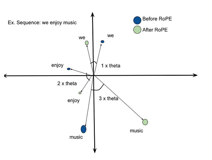
This diagram is the perfect intuition. The vector for "we" (at position 1) is rotated by a small angle θ. The vector for "enjoy" (at position 2) is rotated by 2θ. The vector for "music" (at position 3) is rotated by 3θ.

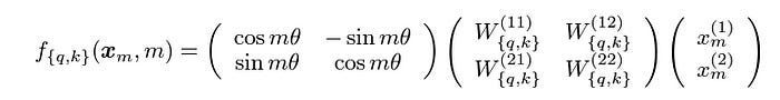
Crucially, the length (magnitude) of the vector doesn't change, only its angle (direction). This rotation is applied to pairs of dimensions within the full Query and Key vectors. Mathematically, this is done by multiplying the vector by a rotation matrix.

The key takeaway is that RoPE injects the absolute position (m) of a token in a way that allows the self-attention mechanism to easily deduce the relative position between any two tokens. It's an incredibly effective and efficient way to give a model a sense of order.

So, what's the problem? The problem arises when this elegant rotation meets the compression mechanism of MLA.

b. The Collision: Why RoPE and Latent Compression Can't Coexist

Let's revisit the core efficiency gain of MLA from Part 1. The reason we can get away with only caching the tiny latent vector c_KV is because we can "pre-calculate" the combined effect of the Key up-projection (W_UK) and the Query up-projection (W_UQ).

During inference, the attention score is calculated based on the Query (q) and the Key (k). In our simplified MLA (without RoPE), this looked like:
Score ∝ q · kᵀ

= (c_q · W_UQ) · (c_KV · W_UK)ᵀ
= c_q · (W_UQ · W_UKᵀ) · c_KVᵀ

Because of the associative property of matrix multiplication, we can pre-compute a new, single matrix W_QK = W_UQ · W_UKᵀ. This allows the query c_q to interact directly with the cached latent vector c_KV via this pre-computed matrix. We never even have to fully reconstruct the Key k! This is the "weight absorption" trick, and it's a huge source of MLA's speed.

Now, let's see what happens when we introduce standard RoPE.

RoPE is applied after the Key vector has been reconstructed. The formula for the Key becomes:
k_with_RoPE = RoPE(c_KV · W_UK)

And the attention score calculation becomes:
Score ∝ q · k_with_RoPEᵀ
= q · (RoPE(c_KV · W_UK))ᵀ

The RoPE() function is a position-dependent rotation matrix (let's call it R) that gets applied inside the parentheses. Our equation now looks something like this:
Score ∝ (c_q · W_UQ) · (R · c_KV · W_UK)ᵀ

When we expand the transpose, this becomes:
Score ∝ c_q · W_UQ · (W_UK)ᵀ · (c_KV)ᵀ · Rᵀ

Look closely. The rotation matrix R is now stuck in the middle of the equation. We can no longer group W_UQ and W_UK together to pre-compute our efficient W_QK matrix. The presence of the R matrix acts as a barrier, breaking the associative property we relied on.

c. The "Tangled" Information and the Broken Optimization

This is the heart of the paradox.

• To be efficient, MLA must be able to absorb the Key's up-projection weights into the Query path.

• To understand word order, the model must apply a position-dependent rotation (RoPE) to its Keys.

• But applying RoPE prevents the weight absorption.

The positional information (the rotation) is "tangled" with the content information (the up-projected vector). By applying RoPE in the standard way, we are forced to fully reconstruct the Key vector for every token in the context window at every single generation step, just to apply the correct rotation.

This completely negates the primary benefit of MLA. We are right back to needing a massive amount of computation, and our dream of a tiny cache and lightning-fast inference is shattered. We've solved the memory problem only to have our solution be incompatible with a feature as fundamental as knowing word order.

So, how do we escape this? How can we apply positional rotation without breaking our beautiful compression scheme? This requires one final, brilliant masterstroke from the DeepSeek team.

Section 3: The Solution: DeepSeek's "Decoupling" Masterstroke

So, we're faced with a frustrating paradox. Our "Master Sketch Artist" (Latent Attention) can create beautifully efficient, compressed sketches of memory, but has no sense of time or order. The tool we use to teach order, RoPE, ruins the sketching process by tangling position with content.

How do we solve this? The team at DeepSeek took a step back and realized the root of the problem was that they were trying to do two jobs with one vector. The Key and Query vectors were responsible for encoding both the content of a token ("what am I?") and its position ("where am I?").

The solution, then, is as brilliant as it is simple in concept: Stop trying to do two jobs with one tool.

This is the "Decoupling" masterstroke. Instead of a single, tangled vector, they decided to create two separate, specialized vectors for both the Query and the Key:

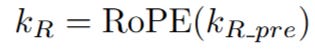
1. A Content Vector (q_C, k_C): This vector is responsible only for the semantic meaning of the token. It is generated using the highly efficient latent compression we learned about in Part 1. It never touches RoPE.

2. A Positional Vector (q_R, k_R): This is a new, smaller vector whose only job is to handle the positional information. RoPE is applied exclusively to this vector.

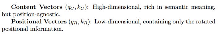
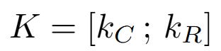
The final Query and Key are then formed by simply concatenating (stitching together) these two separate parts.

Final Query (Q) = Concatenate [Content Query (q_C); Positional Query (q_R)]
Final Key (K) = Concatenate [Content Key (k_C); Positional Key (k_R)]

By separating these concerns, they untangled the knot. The efficient weight absorption trick from Part 1 can be applied to the content part, while the RoPE rotation can be applied independently to the positional part. It's the best of both worlds.

Section 4: The Strategy: Separating Content from Position

a. Our Analogy: The Sketch Artist's Sticky Note

Let's revisit our "Master Sketch Artist" analogy to understand this new strategy.

In Part 1, our artist created a small, information-dense sketch (c_KV) that captured the essence of a scene. This sketch was tiny and efficient to store.

The problem, as we just discovered, is figuring out the order of these sketches. Trying to embed the timestamp or location into the sketch itself (standard RoPE) would warp the drawing and ruin the artist's ability to reconstruct it efficiently.

The Decoupled RoPE solution is equivalent to giving the artist a small sticky note.

1. The Sketch (Content): The artist creates the exact same, efficient black-and-white sketch as before (c_KV -> k_C). This captures the "what."

2. The Sticky Note (Position): On a separate, tiny sticky note, the artist writes down the time and location of the event (h_t -> k_R). This captures the "where" and "when."

3. The Final Record: The detective files the small sketch and the small sticky note together.

When it's time to understand a new clue, the detective doesn't need to ask the artist to redraw a warped sketch. They can show the artist the original content sketch and the positional sticky note separately. The artist can perfectly reconstruct the scene from the sketch while also understanding its context in time from the note.

The content and position are decoupled. They are stored and processed independently until the final moment they are needed, preserving the integrity and efficiency of both.

b. The New Blueprint: Two Parallel Paths for Content and Position

This "sketch and sticky note" strategy gives us a new architectural blueprint. For every input h_t, the information will now flow through three main pathways before the final attention calculation:

1. The Content Path: This is the MLA compression/reconstruction pipeline we learned in Part 1. It creates the content-only q_C and k_C.

2. The Positional Path: A new, parallel path is created to derive the position-only q_R and k_R, and RoPE is applied only here.

3. The Assembly Path: The outputs of these two paths are concatenated to form the final Q and K vectors that are ready for attention.

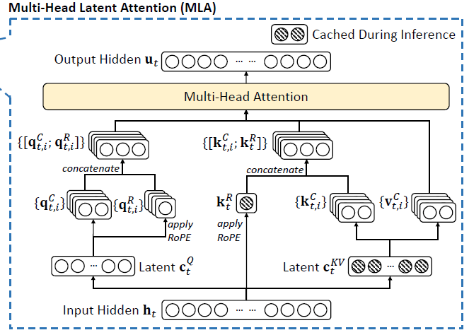
This diagram perfectly illustrates our new blueprint. You can clearly see the Latent c_Q and Latent c_KV paths, and the separate apply RoPE paths that create the k_R and q_R vectors. They all come together right before the final "Multi-Head Attention" step.

Now, let's trace the data through this new, complete blueprint step-by-step.

5. Deep Dive: The Mechanics of Decoupled RoPE

We've established the strategy: separate content from position. Now it's time to roll up our sleeves and trace the data flow through the full Multi-Head Latent Attention architecture, step-by-step. We'll see how the math from the DeepSeek papers translates directly into the computational graph you can explore in the Vizuara AI Lab.

The Setup: Our Input and Learned Weights

Everything begins with our input hidden state, h_t, and a new, expanded set of learned weight matrices. These are the tools our "sketch artist" will use. In addition to the five matrices from Part 1, we now have two new ones specifically for the positional path:

• h_t: The input hidden state (e.g., a 1x8 vector).

• Content Path Weights:

  

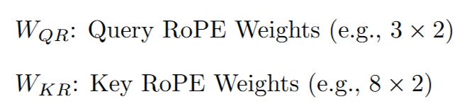
• Positional Path Weights (New):

  

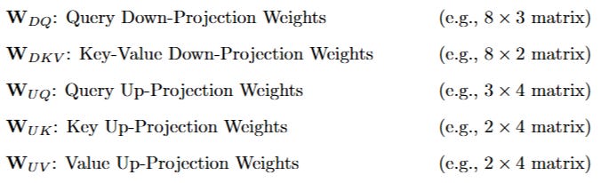
Our mission is to follow h_t as it forks and flows through these matrices to produce the final, complete Query, Key, and Value vectors.

Step 1: The Content Path - Business as Usual

The first part of the process is exactly what we mastered in Part 1. The network calculates the content vectors (q_C and k_C), which are completely free of positional information. This path is all about semantic meaning.

a. Compressing the Input for Query and KV

The input h_t is sent down two parallel compression paths:

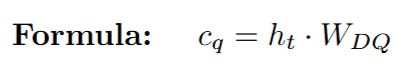
1. Latent Query (c_Q): The input h_t is multiplied by the query down-projection weights W_DQ to create the latent query vector.

   

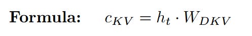
2. Latent Key-Value (c_KV): Simultaneously, h_t is multiplied by the KV down-projection weights W_DKV to create the shared latent sketch for Key and Value. This tiny c_KV vector is the only component from the Key/Value path that will be stored in the cache during inference.

   

b. Reconstructing the Content Vectors

Next, the network reconstructs the full-dimensional content-only vectors from these latent sketches:

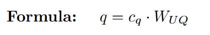
1. Content Query (q_C): The latent query c_Q is multiplied by the query up-projection weights W_UQ.

   

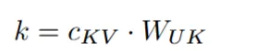
2. Content Key (k_C): The latent sketch c_KV is retrieved (from the cache, during inference) and multiplied by the key up-projection weights W_UK.

   

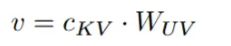
3. Final Value (V): The same latent sketch c_KV is also multiplied by the value up-projection weights W_UV. Note that the Value vector has no positional component, so this is its final form.

   

At the end of this path, we have successfully created q_C, k_C, and V. These vectors are rich in semantic meaning but are completely unaware of their position in the sequence.

Now for the ingenious part. While the Content Path was busy creating the "what" (q_C, k_C), a new, parallel process begins to create the "where" (q_R, k_R). This is the path that will handle the RoPE rotations, keeping them safely separated from our main compression pipeline.

Step 2: The Positional Path - Creating the "Sticky Notes"

This path creates small, specialized vectors whose sole purpose is to be rotated.

a. Deriving the Pre-RoPE Query Vector

The network needs a vector to represent the query's positional aspect. Instead of using the raw input h_t again, it cleverly re-uses the already-computed latent query c_Q. This is efficient and ensures the positional query is derived from the same compressed context as the content query.

This c_Q is multiplied by a new, dedicated weight matrix, W_QR, to create the pre-RoPE query vector, q_R_pre.

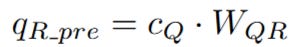
This q_R_pre is a small vector, designed to be the perfect size for the RoPE operation.

b. Deriving the Pre-RoPE Key Vector

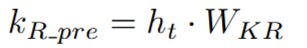
Simultaneously, the network creates the pre-RoPE key vector. Unlike the query, which uses the compressed c_Q, the positional key is derived directly from the original, full hidden state h_t. It is multiplied by another new weight matrix, W_KR. This creates k_R_pre. A crucial point here is that k_R is also cached during inference, alongside c_KV.

At this point, we have two new vectors, q_R_pre and k_R_pre, that are primed and ready for the RoPE rotation. They contain the necessary information, but the positional context has not yet been "injected."

Step 3: Applying RoPE - The Rotation

We now have our pre-positional vectors q_R_pre and k_R_pre. The next step is to inject the positional information by applying the RoPE rotation. As we discussed in Section 2, this is a position-dependent operation. For a token at position m, the rotation is by an angle mθ.

This is represented by the RoPE() function in the DeepSeek paper. In our interactive lab, we simulate this by taking each pair of values [x, y] in the vector and transforming them to [-y, x], which mathematically corresponds to a 90-degree rotation.

1. Apply RoPE to the Query: The pre-RoPE query vector is rotated to produce the final positional query vector, q_R.

   

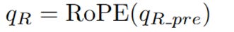
2. Apply RoPE to the Key: The pre-RoPE key vector is rotated to produce the final positional key vector, k_R.

   

Now the magic is complete. We have successfully created two sets of vectors:

Step 4: The Final Assembly - Concatenation

The final step before attention is to assemble our complete Query and Key vectors. This is done via simple concatenation—stitching the content and positional vectors together side-by-side.

1. Final Query (Q):

   

2. Final Key (K):

   

We now have our final Q and K vectors, and the final V vector we derived earlier from the content path. These vectors are now ready for the last step.

Step 5: The Final Attention - A Return to Normalcy

After this intricate dance of compression, reconstruction, and decoupling, the final step is refreshingly simple. We use the exact same standard scaled dot-product attention formula from the original Transformer paper.

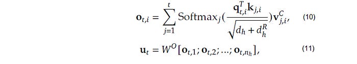
The attention output o_t,i is calculated for each head, and these are combined to produce the final output of the attention block, u_t.

The key difference is in the scaling factor. Because our final Q and K vectors are a concatenation of the content and RoPE parts, their new dimension is d_h_total = d_h_content + d_h_rope. Therefore, we must scale by the square root of this new total dimension.

Scaling Factor = 1 / sqrt(d_h_content + d_h_rope)

And that's it. That is the complete, end-to-end mechanism of Multi-Head Latent Attention with Decoupled RoPE. By cleverly separating the "what" from the "where," the DeepSeek team managed to preserve the massive efficiency gains of latent compression while flawlessly integrating the critical positional information needed for coherent language understanding.

6. The Payoff: Efficiency Without Compromise

We've journeyed through a labyrinth of low-rank projections, latent vectors, and decoupled rotations. While the mathematics are elegant, the true reason this architecture is so revolutionary lies in its staggering real-world impact. By solving the RoPE paradox, MLA with Decoupled RoPE delivers on its promise: it achieves the efficiency of a compressed cache without sacrificing the performance of a full-sized model.

Let's look at the hard numbers from the DeepSeek team's research.

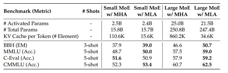
The data in this table is stunning. Across multiple benchmarks and model sizes, MLA consistently shows better performance than standard MHA. This is the holy grail we were looking for. We didn't just match the performance of the memory-hungry MHA; we surpassed it.

This is likely due to the "regularization" effect of the low-rank compression. By forcing the model to pass information through a smaller "bottleneck," it has to learn a more robust and generalized representation of the data, which leads to better performance.

But what about the cache size?

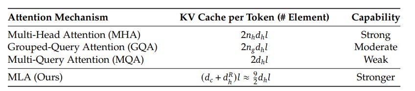
This table shows the ultimate payoff. While achieving stronger performance, MLA requires a significantly smaller amount of KV Cache. For their large model, the cache size using MLA is just 4% of what would be required for standard MHA.

This is not a compromise; it's a complete paradigm shift. We have achieved:

1. Superior Performance: The model is smarter and more capable than its MHA equivalent.

2. Drastically Reduced Memory: The KV Cache is a tiny fraction of its original size, breaking through the memory wall.

This combination unlocks the massive throughput and efficiency gains we saw in Part 1, but now we know it's achieved without any loss of modeling power or positional understanding. It proves that with the right architecture, you don't have to choose between a powerful model and an efficient one. You can have both.

7. Going Deeper: Master Decoupled RoPE in the Vizuara AI Lab!

Theory, diagrams, and equations are one thing, but there is no substitute for seeing the numbers crunch for yourself. To truly internalize how content and position are separated,Understood. Let's bring this home with the final sections. We'll start with the processed, and reassembled, you need to become the computational engine.

That's why we've built the crucial call-to-action for the Vizuara Lab, then provide a powerful, narrative-driven conclusion for the two-part series, and finally, list the references.

Enter the Vizuara AI Lab: Master Decoupled RoPE Now!

8. Conclusion

Our two-part journey began with a critical, often-overlooked challenge in the world of Large Language Models: the memory wall. We saw how the KV Cache, a necessary tool for efficient generation, becomes a massive bottleneck that limits the speed, scale, and economic feasibility of LLMs.

In Part 1, we explored the first layer of the solution: Latent Attention. We followed the strategy of the "Master Sketch Artist," who compresses high-dimensional memories into tiny, efficient latent sketches, solving the core memory problem. We achieved staggering efficiency gains but were left with a crucial cliffhanger: our solution was position-agnostic.

In this post, we confronted that final challenge head-on. We discovered the RoPE Paradox how standard positional embeddings would tangle with our compression mechanism and break its efficiency. The solution was a final, elegant masterstroke: Decoupled RoPE. By separating a token's "what" (content) from its "where" (position), the architecture preserves the best of both worlds.

We have now seen the complete picture. Multi-Head Latent Attention is a beautiful synthesis of ideas:

1. It uses low-rank projections to compress Keys and Values into a tiny latent cache, solving the memory bottleneck.

2. It uses a decoupled architecture to handle positional information separately, solving the RoPE paradox.

The result is an attention mechanism that is not only more memory-efficient and faster during inference but is also more powerful and performant than its predecessors. It is a testament to the fact that the most profound breakthroughs often come not just from scaling up, but from fundamentally rethinking the problem. You now understand the mechanics of one of the most important architectural innovations driving the future of efficient, large-scale AI.

9. References

This series is a conceptual deep dive inspired by the groundbreaking work of researchers and engineers in the AI community. For those wishing to explore the source material and related concepts further, we highly recommend the following papers and resources:

• [1] DeepSeek-AI. (2024). DeepSeek-V2: A Strong, Economical, and Efficient Mixture-of-Experts Language Model. arXiv:2405.04434

• [2] Liu, A., Feng, B., et al. (2024). Deepseek-v3 technical report. arXiv:2412.19437

• [3] Vaswani, A., Shazeer, N., et al. (2017). Attention Is All You Need. arXiv:1706.03762

• [4] Shazeer, N. (2019). Fast Transformer Decoding: One Write-Head is All You Need. arXiv:1911.02150

• [5] Ainslie, J., Lee-Thorp, J., et al. (2023). GQA: Training Generalized Multi-Query Transformer Models from Multi-Head Checkpoints. arXiv:2305.13245

Stay Connected

So.. that's all for today.

Follow me on LinkedIn and Substack for more such posts and recommendations, till then happy Learning. Bye👋