Decoding Naive Bayes: From Word Counts to Smart Predictions

Uncover the simple yet powerful math of probability that powers spam filters and text classifiers. Discover how Bayes' Theorem and a "naive" assumption let us predict outcomes with stunning accuracy.

Table of content

1. Introduction: The World of Probabilistic Decisions

2. The Foundation: The Power of Bayes' Theorem

3. The "Naive" Assumption: Simplicity for Power

4. How Naive Bayes Works: A Step-by-Step Walkthrough

5. The Verdict: Advantages and Limitations

6. Going Deeper: Implement Naive Bayes in the Vizuara AI Lab!

7. Conclusion

8. References

1. Introduction: The World of Probabilistic Decisions

Think about how you make decisions every day. It's often a game of probabilities. When you step outside, you might glance at the sky and think, "Those dark clouds look like rain." You don't know for sure, but based on past experiences" dark clouds often mean rain" you make a probabilistic judgment. Or perhaps you receive an email. Your brain instantly flags certain words or phrases "win big," "urgent action," "free money" and you instinctively classify it as spam, even before you consciously analyze every word.

This is the essence of thinking in probabilities: weighing evidence and making a judgment about the likelihood of an event or category. In our previous deep dives, we've equipped our machines with powerful tools for prediction and classification. We taught them to draw lines to predict continuous values with Linear Regression, to bend those lines into 'S' shapes to predict "Yes" or "No" probabilities with Logistic Regression, and even to understand complex patterns in images with CNNs or remember long conversations with Transformers.

But what if the problem isn't about finding a complex hidden relationship, or a perfect S-curve, or intricate visual features? What if the problem is fundamentally about likelihood? About directly answering: "Given this evidence, what is the probability that it belongs to this category?"

This is a different kind of classification, one rooted deeply in the elegant mathematics of chance. It's how some of the simplest yet most effective machine learning algorithms work, constantly weighing the odds. Today, we're going to pull back the curtain on one such foundational algorithm, a true classic in machine learning that makes incredibly "smart predictions" from surprisingly simple "word counts." Its name is Naive Bayes.

2. The Foundation: The Power of Bayes' Theorem

At the heart of Naive Bayes lies a theorem that has revolutionized how we think about probability and inference: Bayes' Theorem. It's a formula that allows us to update our beliefs about an event based on new evidence. In essence, it answers the question: "What is the probability of an event A happening, given that event B has already happened?"

This isn't just abstract math; it's the core logic behind how we make informed decisions in the face of uncertainty. For example:

• What is the probability that an email is spam (A), given that it contains the word "viagra" (B)?

• What is the probability that a patient has a disease (A), given that they tested positive (B)?

• What is the probability that a day is good for playing golf (A), given that the weather is sunny (B)?

Bayes' Theorem provides a rigorous way to calculate these "posterior probabilities" (P(A|B)) by combining prior knowledge (P(A)) with new evidence (P(B|A) and P(B)).

Formula for Bayes' Theorem:

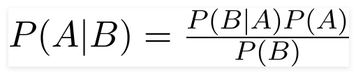
Let's break down each component:

• P(A|B): The Posterior Probability

  • This is what we want to find. It's the probability of our Hypothesis (A) being true, given the Evidence (B). For example, the probability that the email is spam, given the word "viagra" is present.

• P(B|A): The Likelihood

  • This is the probability of seeing the Evidence (B), given that our Hypothesis (A) is true. For example, the probability of the word "viagra" appearing, if the email is spam.

• P(A): The Prior Probability

  • This is our initial belief, the probability of our Hypothesis (A) being true before we see any evidence. For example, the general probability of any email being spam (e.g., 10% of all emails are spam, regardless of content).

• P(B): The Marginal Probability (or Evidence Probability)

  • This is the overall probability of seeing the Evidence (B), regardless of the hypothesis. For example, the general probability of the word "viagra" appearing in any email (spam or not spam). It acts as a normalizing factor.

So, Bayes' Theorem can be intuitively understood as:
Posterior Probability = (Likelihood * Prior Probability) / Evidence Probability

It tells us: "How likely is our hypothesis, given the evidence, compared to just how likely the evidence is overall?"

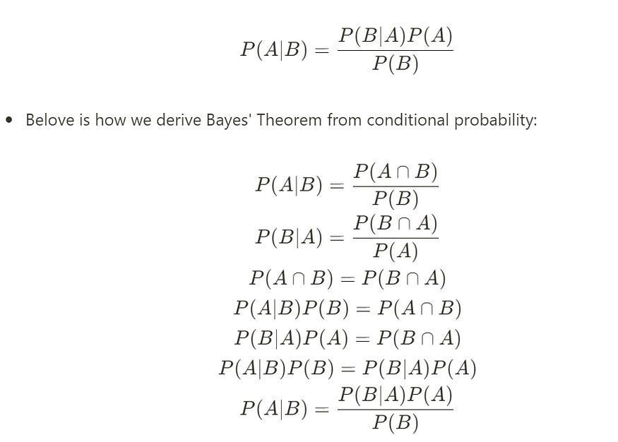
Now, let's briefly look at how this theorem is derived from the fundamental rules of conditional probability.

The beauty of Bayes' Theorem isn't just in its utility, but also in its elegant simplicity. It's not a magical formula that appeared out of nowhere; it's logically derived directly from the fundamental rules of conditional probability.

Let's trace this derivation step-by-step.

Step 1: Define Conditional Probability

Conditional probability is the probability of an event occurring given that another event has already occurred. For two events, A and B:

• The probability of event A occurring given that event B has occurred is:
  P(A|B) = P(A ∩ B) / P(B)
  (This means: the probability of A and B both happening, divided by the probability of B happening alone.)

• Similarly, the probability of event B occurring given that event A has occurred is:
  P(B|A) = P(B ∩ A) / P(A)
  (This means: the probability of B and A both happening, divided by the probability of A happening alone.)

Step 2: Recognize the Commutative Property of Intersection

The event of "A and B both happening" (A ∩ B) is the same as the event of "B and A both happening" (B ∩ A). Therefore:

P(A ∩ B) = P(B ∩ A)

Step 3: Rearrange the Second Conditional Probability Equation

From our second conditional probability definition (P(B|A) = P(B ∩ A) / P(A)), we can multiply both sides by P(A) to isolate P(B ∩ A):

P(B ∩ A) = P(B|A) * P(A)

Step 4: Substitute and Conclude

Now, we take this rearranged expression for P(B ∩ A) and substitute it back into the very first conditional probability definition (P(A|B) = P(A ∩ B) / P(B)), since we know P(A ∩ B) is equal to P(B ∩ A):

P(A|B) = [P(B|A) * P(A)] / P(B)

And there you have it! This simple substitution reveals the elegant truth of Bayes' Theorem. It shows how our initial knowledge (P(A)), combined with new evidence (P(B|A) and P(B)), allows us to precisely calculate a revised probability (P(A|B)). This foundational principle is what gives Naive Bayes its remarkable ability to classify.

3. The "Naive" Assumption: Simplicity for Power

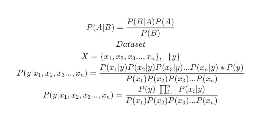
Nayes' Theorem provides a beautiful framework for calculating P(Hypothesis | Evidence). In classification, our Hypothesis (y) is the class we want to predict (e.g., "spam," "not spam," "positive sentiment"), and our Evidence is the set of features (x1, x2, ..., xn).

Our ultimate goal is to calculate P(y | x1, x2, ..., xn) the probability of a certain class y, given the specific set of features we've observed.

Using Bayes' Theorem, we can express this as:

P(y | x1, ..., xn) = [P(x1, ..., xn | y) * P(y)] / P(x1, ..., xn)

Let's re-state our terms with this correct formula in mind:

• Posterior P(y | x1, ..., xn): What we want to calculate. The probability of a class y given our set of features.

• Likelihood P(x1, ..., xn | y): The probability of observing this specific combination of features, given that the class is y.

• Prior P(y): The overall probability of class y.

• Evidence P(x1, ..., xn): The overall probability of observing this combination of features.

a. The Problem: The Intractable Likelihood

We've arrived back at the same practical problem, but let's state it with precision. The Likelihood term, P(x1, x2, ..., xn | y), is the real challenge.

Calculating this joint probability is incredibly difficult. It requires understanding the complex, interdependent relationships between all the features. Does the presence of the word "viagra" (x1) make the presence of the word "money" (x2) more likely within spam emails? Does "sunny" weather (x1) affect the probability of "high humidity" (x2) on days when we play golf?

To calculate this term correctly, we would need a massive dataset that contains examples of every possible combination of features for every class. This is computationally expensive and, in most real-world scenarios, completely infeasible. We'd need an impossibly large amount of data.

This is where the "naive" assumption comes in to save the day, turning an intractable problem into a beautifully simple one.

b. The Solution: Assuming Independence (and Why it Works "Naively")

The Naive Bayes classifier gets its name from the one, giant, simplifying leap of faith it takes. It makes the "naive" assumption of conditional independence.

It assumes that, for a given class y, every feature is completely independent of every other feature.

In other words, it assumes:

• The probability of an email containing the word "viagra" has absolutely no effect on the probability of it also containing the word "money," as long as we know it's a spam email.

• The probability of the weather being "sunny" has no effect on the probability of the humidity being "high," as long as we know it's a day we're playing golf.

This is obviously not true in the real world. Words in a language are highly dependent on each other. But this assumption is incredibly powerful because it allows us to break down the impossible joint likelihood term into a set of simple, individual probabilities.

Thanks to the rules of probability, if we assume features x1 and x2 are independent, we can say:

P(x1, x2) = P(x1) * P(x2)

Applying this assumption to our likelihood term P(x1, x2, ..., xn | y), we can break it apart:

P(x1, x2, ..., xn | y) = P(x1|y) * P(x2|y) * ... * P(xn|y)

This is a monumental simplification! Instead of calculating one impossibly complex joint probability, we now only need to calculate the individual probability of each feature occurring, given the class. These individual probabilities are easy to compute directly from our training data by just counting frequencies.

c. The Naive Bayes Classification Formula

With this assumption in place, our full Bayes' Theorem equation transforms.

The original formula:
P(y | x1, ..., xn) = [P(x1, ..., xn | y) * P(y)] / P(x1, ..., xn)

Becomes:
P(y | x1, ..., xn) = [P(x1|y) * P(x2|y) * ... * P(xn|y) * P(y)] / P(x1, ..., xn)

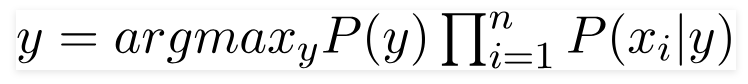
This can be written more compactly using the Pi (Π) notation for products:
P(y | x1, ..., xn) = [P(y) * Π P(xi|y)] / P(x1, ..., xn)

This is the complete formula for the Naive Bayes classifier. To make a prediction, we calculate this value for every possible class (y). For example, we calculate P(spam | features) and P(not spam | features).

Notice that the denominator, P(x1, ..., xn), is the same for all classes. It's a constant normalizing factor. Since we only care about which class has the highest probability, we can often ignore the denominator and just compare the numerators:

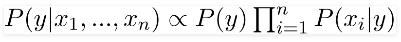
The class y that gives the highest value for this calculation is our final prediction. This is known as Maximum A Posteriori (MAP) estimation.

Despite its "naive" assumption, this simple and elegant formula is remarkably effective and forms the basis of highly successful classifiers, especially for text.

4. How Naive Bayes Works: A Step-by-Step Walkthrough

The theory is elegant, but the real beauty of Naive Bayes is how simple it is to apply in practice. It's an algorithm you can almost perform with a pen and paper. Let's walk through a classic example to see exactly how it works.

a. Scenario 1: A Numerical Example (Playing Golf)

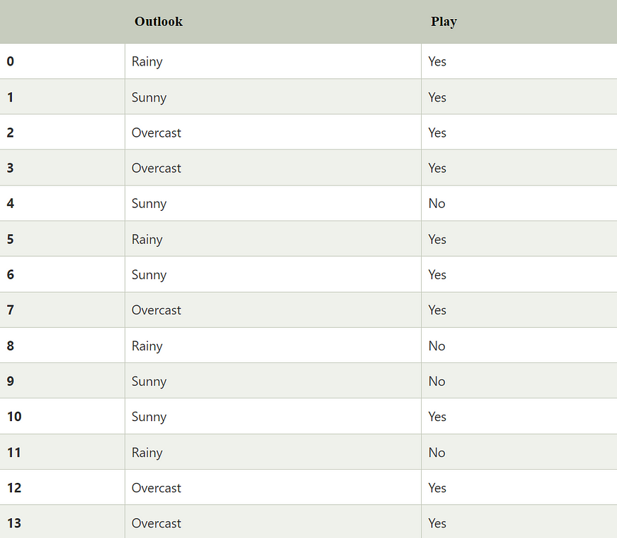
Imagine we're a groundskeeper at a golf course, and we want to predict whether people will play golf on a given day based on the weather outlook. We have a small dataset of past observations.

The Problem:
A new day arrives, and the outlook is Sunny. Will the players show up?
Our goal is to calculate:

1. P(Play=Yes | Outlook=Sunny)

2. P(Play=No | Outlook=Sunny)

We will then choose the class with the higher probability as our prediction.

Step 1: Calculate the Prior Probabilities, P(y)

First, we ignore the evidence (the weather) and just calculate the overall probability of each class from our dataset of 14 days.

• P(Play=Yes): Out of 14 days, people played on 10 of them.
  P(Yes) = 10 / 14 = 0.71

• P(Play=No): Out of 14 days, people did not play on 4 of them.
  P(No) = 4 / 14 = 0.28

Step 2: Calculate the Likelihoods, P(Evidence | Class)

Now, we calculate the probability of our evidence ("Sunny") occurring for each class.

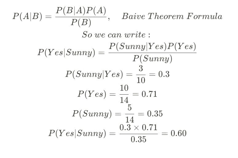
• P(Outlook=Sunny | Play=Yes): We look only at the 10 days where people played (Play=Yes). Out of these 10 days, how many were Sunny? The answer is 3.
  P(Sunny | Yes) = 3 / 10 = 0.3

• P(Outlook=Sunny | Play=No): We look only at the 4 days where people did not play (Play=No). Out of these 4 days, how many were Sunny? The answer is 2.
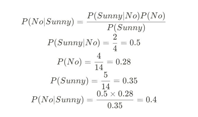
  P(Sunny | No) = 2 / 4 = 0.5

Step 3: Calculate the Marginal Probability of the Evidence, P(Evidence)

We need the overall probability of the weather being "Sunny," regardless of whether people played or not.

• P(Outlook=Sunny): Out of the 14 total days, 5 were Sunny.
  P(Sunny) = 5 / 14 = 0.35

Step 4: Apply Bayes' Theorem

Now we have all the pieces to plug into our formula P(y | X) = [P(X | y) * P(y)] / P(X).

• For the "Yes" class:
  P(Yes | Sunny) = [P(Sunny | Yes) * P(Yes)] / P(Sunny)
  P(Yes | Sunny) = (0.3 * 0.71) / 0.35 = 0.60

• For the "No" class:
  P(No | Sunny) = [P(Sunny | No) * P(No)] / P(Sunny)
  P(No | Sunny) = (0.5 * 0.28) / 0.35 = 0.4

The Verdict:

The probability of people playing golf given a sunny day is 0.60.
The probability of people not playing golf given a sunny day is 0.40.

Since 0.60 > 0.40, our Naive Bayes classifier predicts Yes, people will play golf. It's that simple a series of counts and divisions leads to an intelligent, probabilistic prediction.

b. Scenario 2: A Text Classification Example (Sentiment Analysis)

Let's use Naive Bayes to determine if a sentence has positive or negative sentiment. This is the core logic behind many spam filters and basic sentiment analysis tools.

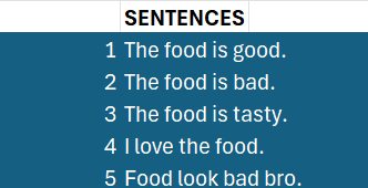
First, imagine we have a small dataset of sentences that have already been labeled as positive (1) or negative (0).

Step 1: Text Preprocessing and Feature Representation

Before a computer can work with text, we need to convert it into numbers. This involves two sub-steps:

1. Preprocessing: We clean the text by converting it to lowercase, removing punctuation, and often removing common "stop words" (like "is," "the," "a") that don't carry much meaning. For our example, "The food is good." becomes food good.

2. Feature Representation (Bag of Words): We then convert these sentences into numerical vectors. A simple and effective way to do this is with the Bag of Words model. We create a vocabulary of all the unique words in our dataset (e.g., food, good, love, tasty, bad). Then, for each sentence, we create a vector that marks the presence (1) or absence (0) of each word from our vocabulary.

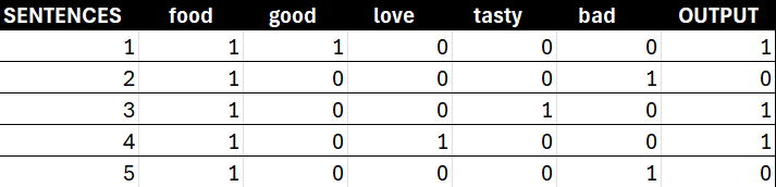
Our dataset is now in a numerical format that our algorithm can understand.

The Problem:
We get a new, unseen sentence: "The food is good". After preprocessing, this becomes food good. Is this sentence positive (y=1) or negative (y=0)?

Our features are x1 = food and x2 = good. We need to calculate P(y=1 | "food good") and P(y=0 | "food good") and see which is higher.

Step 2: Apply the Naive Bayes Formula

Let's start by calculating the probability that the sentence is positive (y=1).

Our formula, thanks to the naive assumption, is:
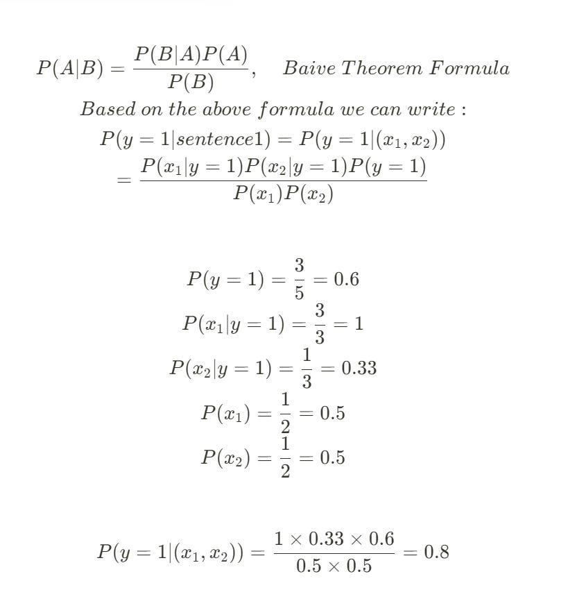
P(y=1 | "food good") = [P(food|y=1) * P(good|y=1) * P(y=1)] / P("food good")

Let's calculate each term from our training data:

• Prior P(y=1): Out of 5 sentences, 3 are positive.
  P(y=1) = 3 / 5 = 0.6

• Likelihood P(food | y=1): Look only at the 3 positive sentences. All 3 of them contain the word "food."
  P(food | y=1) = 3 / 3 = 1.0

• Likelihood P(good | y=1): Look only at the 3 positive sentences. Only 1 of them contains the word "good."
  P(good | y=1) = 1 / 3 = 0.33

Now, let's calculate the numerator:
Numerator = 1.0 * 0.33 * 0.6 = 0.198

Now, let's do the same for the negative (y=0) class.

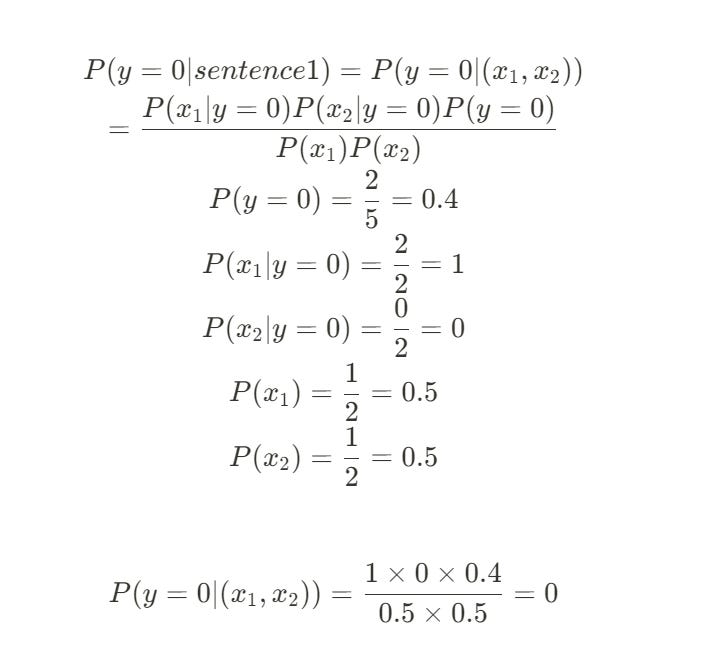
• Prior P(y=0): Out of 5 sentences, 2 are negative.
  P(y=0) = 2 / 5 = 0.4

• Likelihood P(food | y=0): Look only at the 2 negative sentences. Both of them contain the word "food."
  P(food | y=0) = 2 / 2 = 1.0

• Likelihood P(good | y=0): Look only at the 2 negative sentences. Zero of them contain the word "good."
  P(good | y=0) = 0 / 2 = 0.0

Now, let's calculate the numerator for the negative class:
Numerator = 1.0 * 0.0 * 0.4 = 0

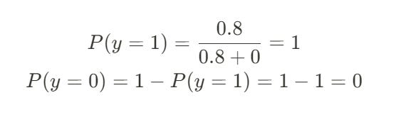
The Verdict (Unnormalized):
The score for the positive class is 0.198.
The score for the negative class is 0.

Since 0.198 > 0, the model predicts the sentence is Positive.

An Important Note on Zeros (Laplace Smoothing):
Notice we got a probability of 0 for P(good | y=0). This can be dangerous. If a word simply doesn't appear in a class in our training data, it will make the entire probability for that class zero, which might not be accurate. To fix this, a simple technique called Laplace (or Additive) Smoothing is used. We add a small number (usually 1) to every count, so no probability can ever be exactly zero.

The result will be the same. The model is 100% confident the sentence is positive based on our small dataset.

5. The Verdict: Advantages and Limitations

We've journeyed through the elegant, probability-driven world of the Naive Bayes classifier. We've seen how a theorem from the 18th century, combined with a pragmatic "naive" assumption, creates a powerful and surprisingly effective algorithm for classification. But like any tool, it has its specific strengths and weaknesses. Understanding these is key to knowing when to reach for Naive Bayes in your machine learning toolkit.

The Advantages: Why Naive Bayes Endures

1. Incredibly Fast and Efficient: This is perhaps its greatest strength. The training process for Naive Bayes is not an iterative optimization like Gradient Descent. It consists of simply calculating frequencies from the training data. This makes it lightning-fast, even on very large datasets.

2. Simple and Easy to Implement: The logic is straightforward. As we've seen, you can almost perform the calculations by hand. This makes it a fantastic baseline model to quickly get a sense of a classification problem's difficulty.

3. Works Well with High-Dimensional Data: Naive Bayes shines in scenarios with a huge number of features, like text classification, where the "vocabulary" can run into the tens of thousands. While models like Logistic Regression might struggle, Naive Bayes handles this "curse of dimensionality" with ease.

4. Requires Less Training Data: Compared to more complex models that need to learn intricate relationships, Naive Bayes can often achieve decent performance with a surprisingly small amount of training data.

5. Good at Handling Categorical Features: It naturally works with categorical data (like "Sunny," "Rainy," "Overcast") without needing complex transformations.

The Limitations: The Price of Naivety

1. The "Naive" Assumption is (Almost) Always Wrong: This is the algorithm's Achilles' heel. In the real world, features are rarely independent. The word "San" is highly dependent on the word "Francisco." This violation of its core assumption means Naive Bayes may not capture complex relationships in the data.

2. Known to be a Bad Estimator: While Naive Bayes is a good classifier (it's good at picking the most likely class), the actual probability scores it outputs (P(y|X)) can be unreliable. Because of the strong independence assumption, these probabilities tend to be pushed towards 0 or 1. So, you should trust its final prediction, but not necessarily the confidence score it gives you.

3. The Zero-Frequency Problem: As we touched upon, if a feature in the test data was never seen in the training data for a particular class, the model will assign it a zero probability, wiping out all other information. This must be addressed with a smoothing technique like Laplace smoothing.

4. Sensitivity to Irrelevant Features: If you include features that have no predictive power, they can still "pollute" the calculation by adding noise to the probability estimates, potentially harming the model's performance.

In summary, Naive Bayes is a brilliant, efficient, and often surprisingly powerful "first-line-of-defense" classifier. Its simplicity is its greatest asset, but also the source of its primary limitation. It's a testament to the power of sound probabilistic reasoning and remains a vital tool for any data scientist.

6. Going Deeper: Implement Naive Bayes in the Vizuara AI Lab!

That's why we've built the next chapter of our learning series in the Vizuara AI Lab. This isn't a code-along where you just type; it's a hands-on environment where you become the computational engine of the Naive Bayes classifier. In our lab, you will:

• Manually calculate Prior probabilities from a dataset.

• Compute the Likelihood for different features and classes step-by-step.

• Apply Bayes' Theorem to combine your calculated probabilities and make a final prediction.

• Witness the "naive" assumption in action as you multiply independent probabilities together.

Reading is knowledge. Calculating is understanding. Are you ready to master the simple power of probabilistic classification?

Enter the Vizuara AI Lab: Build Your First Naive Bayes Classifier Now!

7. Conclusion

Our journey began with a simple observation: much like us, machines can learn to make intelligent judgments based on the likelihood of events. We explored how the principles of probability, codified in the 18th-century Bayes' Theorem, provide a powerful framework for this kind of reasoning.

We saw how this elegant theorem, when combined with a pragmatic but powerful "naive" assumption of feature independence, transforms into a practical and incredibly efficient classification algorithm. We walked through the process step-by-step, seeing how simple counts of words or weather conditions can be converted into robust probabilistic predictions.

The shift from complex, iterative optimization models like Logistic Regression to the direct, frequency-based calculations of Naive Bayes highlights a core truth in machine learning: there is often more than one way to solve a problem. Naive Bayes is a testament to the fact that sometimes, the most profound breakthroughs come not from increasing complexity, but from the clever and elegant application of first principles.

You now understand the core engine behind spam filters, basic sentiment analyzers, and a whole class of powerful diagnostic tools. You've decoded another fundamental pillar of machine learning, one built not on finding a line, but on a deep understanding of chance.

8. References

• [1] Bayes' Theorem, Stanford Encyclopedia of Philosophy. (A comprehensive look at the history and philosophy behind the theorem.)

• [2] Shubh Tripathi (2023). Naive Bayes Classifiers, Medium. (A clear, practical guide with code examples.)

• [3] Fraidon Omarzai (2023). Naive Bayes Algorithm In-depth, Medium. (Another excellent tutorial that breaks down the concepts.)

• [4] Manning, P., Raghavan, P., & Schütze, H. (2008). Introduction to Information Retrieval. Cambridge University Press. (Chapter 13 provides a classic, in-depth explanation of Naive Bayes for text classification.)

Stay Connected

So.. that's all for today.

Follow me on LinkedIn and Substack for more such posts and recommendations, till then happy Learning. Bye👋