


Decoding RNNs: How Neural Networks Gain Memory for Sequences
Discover how these neural networks gain the ability to remember previous inputs, unlocking capabilities for language modeling, prediction, and understanding sequential data.

Table of content
Introduction: The Need for Memory
The Problem with Feedforward Networks for Sequences
The Solution: Enter Recurrent Neural Networks!
Deep Dive into RNNs (Theory)
What Are RNNs Used For? (Common Applications)
Beyond Simple RNNs
Going Deeper: Explore the Mechanics with the Vizuara AI Learning Lab!
Conclusion
1. Introduction: The Need for Memory
In our previous blog post, "Decoding CBOW: How Neural Networks Learn Word Embeddings by Filling in the Blanks", we peeled back the curtain on how neural networks can learn rich, dense representations of words – word embeddings! We saw how models like CBOW cleverly leverage the context of surrounding words within a fixed window to understand meaning. This was a massive leap beyond simple one-hot encoding, allowing computers to grasp semantic relationships like synonyms and analogies. Pretty cool, right?
But here’s the thing. While CBOW and similar models are great at understanding words based on their immediate neighbors, they have a significant limitation: they don't have a memory of the sequence itself. They look at a small, isolated window of words.
Think about how we understand language. When you read a sentence, or listen to someone speak, you don't just process the current word and its immediate neighbors. Your brain keeps track of what came before. You remember the subject of the previous sentence, the setting of the story, or the topic of the conversation. This accumulated knowledge, this "memory" of the sequence, is absolutely crucial for true understanding.

ht) from one time step to the next, enabling sequential processing.Consider these two sentences:
The dog chased the cat. It ran fast.
The dog barked at the mailman. It ran fast.
As humans, we effortlessly understand that in the first sentence, "It" refers to the cat (because cats typically run fast when chased by dogs!), while in the second sentence, "It" likely refers to the mailman (because mailmen often run when barked at by dogs!). How do we know this? Because we processed the sentences sequentially, keeping track of the subjects and actions. We used our memory of the earlier words to understand the meaning of "It" later in the sequence.
Standard feedforward neural networks or fixed-window models like basic CBOW struggle immensely with this kind of sequential dependency. They lack the mechanism to carry information forward from one step (or word) to the next.
So, how do we build neural networks that can remember? How do we give them the power to process sequences, where the order of inputs matters, and past information influences the processing of future inputs?
This is where Recurrent Neural Networks (RNNs) enter the picture! RNNs are specifically designed to handle sequential data by incorporating an internal state or "memory" that persists across time steps.

2. The Problem with Feedforward Networks for Sequences
As we highlighted the crucial need for memory when processing sequential data like language or time series. We contrasted the conceptual structure of a standard feedforward network with that of a recurrent one. Now, let's really hammer home why traditional feedforward networks fundamentally fall short for these kinds of tasks.
Think back to any feedforward network you've encountered – perhaps the one we built for CBOW (ignoring the context averaging part for a moment, just the input-to-output layers) or a simple image classifier. Data flows in one direction only, from the input layer through hidden layers to the output layer. Each input instance is processed independently of any other.
This architecture is great for tasks where each data point is self-contained, like classifying an image or predicting a house price based on a fixed set of features. But for sequences, it creates major headaches:
No Memory of the Past: This is the biggest issue. A feedforward network processing a word in a sentence has no inherent way of knowing what words came before it in that same sentence. When it sees "It" in "The dog chased the cat. It ran fast.", it sees "It" in isolation (or within a tiny, fixed window that might miss the key word "cat"). It doesn't retain any information about the dog or the cat from the previous parts of the sequence. The state is reset with every new input.
Fixed Input Size: Feedforward networks are designed to accept inputs of a fixed size. If your network takes 10 features for a house price prediction, you must always give it exactly 10 features. How do you apply this to sentences or sequences that can be of any length? You'd need a different network for every possible sentence length, or you'd have to pad shorter sequences and truncate longer ones, which is awkward and inefficient. It's like trying to process paragraphs by only ever looking at exactly 5 words at a time, no more, no less.
No Parameter Sharing Across Time: Imagine you could feed a whole sentence into a giant feedforward network. You might have weights connecting the first word's input features to the first hidden layer, the second word's features to the first hidden layer, and so on. But the weights used for the first word would likely be different from the weights used for the second, third, or tenth word. However, the operation of processing a word should ideally be consistent regardless of its position in the sequence. Feedforward nets don't naturally share these processing weights across the time steps of a sequence.
In short, standard feedforward networks are designed for static data, not dynamic, ordered sequences where the context builds over time. They are blind to the flow and dependencies that make sequential data meaningful. This is precisely the gap that Recurrent Neural Networks were invented to fill.
3. The Solution: Enter Recurrent Neural Networks!
We've laid out the problem: feedforward networks, for all their power, hit a wall when it comes to understanding data that unfolds over time. They lack memory, they struggle with variable-length inputs, and they can't easily apply the same processing logic consistently across a sequence. So, how do we fix this fundamental blind spot?
The answer, elegantly simple yet profoundly powerful, lies in Recurrent Neural Networks (RNNs).
Imagine you're taking notes during a lecture. You write down the current point, but you also glance back at your previous notes to make sure everything connects. That's essentially what an RNN does!
The core innovation of an RNN is its internal loop. Unlike a feedforward network that's a straight shot from input to output, an RNN includes a connection that feeds the output (or, more precisely, an internal "hidden state") from the previous time step back into the network as an input for the current time step.
This looping mechanism allows the network to:
Develop a "Memory": At each step in a sequence, the RNN takes the current input (e.g., a word) and combines it with its "memory" of what it processed in the previous steps. This memory isn't a perfect recollection, but a distilled, continuously updated summary of the sequence seen so far. It's often referred to as the hidden state.
Process Variable-Length Sequences: Because the network simply iterates over the sequence, one element at a time, it can handle inputs of almost any length. It's like having a single processing unit that you just keep feeding data to, and it keeps updating its internal state.
Share Parameters Across Time: Crucially, the same set of weights and biases are applied at every single time step within the loop. This means the network learns a universal way to transform input and update its hidden state, no matter where in the sequence that transformation occurs. This parameter sharing is incredibly efficient and helps the model generalize patterns across the entire sequence.
In essence, RNNs introduce the concept of "time" or "sequence" into neural network architectures. They allow information to persist and be influenced by past observations, giving them a remarkable ability to understand context, predict future elements, and generate coherent sequences – whether it's predicting the next word in your sentence, generating music, or understanding stock market trends.
This is the fundamental shift, moving us from processing isolated data points to truly understanding the flow and dependencies within sequential information. Now that we've grasped the core idea of the loop, we're ready to peel back another layer and look at the actual mechanics of how this "memory" works and gets updated.
4. Deep Dive into RNNs (Theory)
In our previous sections, we established the critical need for memory in neural networks that process sequential data. We saw how traditional feedforward networks are fundamentally amnesiac, treating each input in isolation. We then introduced the Recurrent Neural Network (RNN) as the architectural solution, highlighting its internal loop as the conceptual source of this memory.
Now, it's time to pull back the curtain and get our hands dirty with the mechanics. We'll explore the intricate mathematical operations that govern an RNN's behavior, see how information actually flows through time, and understand how it learns to connect the dots in a sequence.
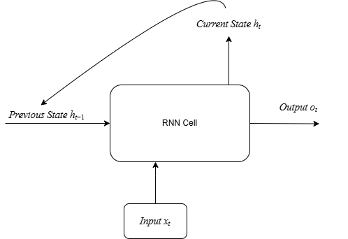
At the heart of every RNN is its fundamental building block, often called the "RNN cell" or "recurrent unit." This cell is the engine that performs the computation for a single time step in the sequence. What makes it "recurrent" is its unique ability to take two inputs: the new piece of information from the current time step, and a summary of everything it has seen before. This summary is its "memory."
Let's define the key components and their roles at a given time step, which we'll call t:
Input (x(t)): This is the data for the current moment in the sequence. If we're processing a sentence character by character, x(t) would be the vector representation (like a one-hot vector) for the character at position t.
Previous Hidden State (a(t-1)): This is the memory from the immediately preceding time step. It's a vector that encapsulates a summary of all previous inputs up to t-1. This is the revolutionary ingredient that feedforward networks lack. For the very first time step (t=1), since there is no previous memory, we typically initialize this as a vector of all zeros.
Current Hidden State (a(t)): This is the new, updated memory of the network after it has processed the input at time t. It's calculated by combining the previous hidden state a(t-1) with the current input x(t). This new state will then be passed on to the next time step, t+1, to become its "previous hidden state."
Output (y_hat(t)): This is the prediction or output generated by the network at the current time step t. This prediction is based entirely on the information contained in the current hidden state, a(t).

The Math of the Forward Pass: How Memory and Predictions are Made
Now let's look at the two crucial calculations that happen inside the RNN cell during the forward pass. These are the exact steps the network takes to update its memory and make a prediction.
4.1 Updating the Hidden State (Creating the New Memory)
The most important job of the RNN cell is to intelligently merge the old memory with the new information. It needs to decide what to keep from the past and what to add from the present. This is not just a simple addition; it's a learned transformation controlled by weights.
The formula for this update is:
a(t) = tanh(W_aa * a(t-1) + W_ax * x(t) + b_a)
Let's break that down piece by piece:
W_ax * x(t): The network takes the current input x(t) and multiplies it by a weight matrix called W_ax. This matrix controls the importance of the new input. The network learns the values for W_ax during training, essentially learning how much to "listen" to the new information.
W_aa * a(t-1): Simultaneously, the network takes the memory from the previous step, a(t-1), and multiplies it by a different weight matrix, W_aa. This matrix governs the influence of the past. By learning W_aa, the network figures out how much of its old memory it should retain.
... + b_a: These two results are added together, along with a bias term, b_a. A bias allows the network to shift the result up or down, giving it more flexibility.
tanh(...): The entire sum is then passed through a non-linear activation function, typically the hyperbolic tangent (tanh). This is critical. Without a non-linear function, the RNN would just be a series of linear operations, which is not powerful enough to learn complex patterns in data like language. The tanh function also has the convenient property of squashing all the values to be between -1 and 1, which helps keep the numbers in the network from exploding or vanishing.
The result of this entire operation, a(t), is the new hidden state the network's updated understanding of the sequence up to this point.
4.2 Calculating the Output (Making a Prediction)
Once the cell has computed its new hidden state a(t), it has everything it needs to make a prediction for the current time step. The output is a direct function of this new, updated memory. This makes intuitive sense: your prediction at any given moment should be based on your complete understanding of the context so far.
The formula for calculating the output is:
y_hat(t) = softmax(W_ya * a(t) + b_y)
Let's dissect this one as well:
W_ya * a(t): The network takes the newly calculated hidden state a(t) and multiplies it by an output weight matrix, W_ya. This matrix's job is to translate the internal memory representation into something that is meaningful for the desired output. For example, it learns to convert the abstract features of the memory into scores for each possible next character in a vocabulary.
... + b_y: Just like before, a bias term b_y is added to provide more flexibility to the output transformation. The result of this addition is often called the "logits" – the raw, unnormalized scores for each possible class.
softmax(...): The logits are then passed through a softmax activation function. This is an extremely useful function for classification tasks. It takes a vector of arbitrary real-numbered scores and transforms it into a probability distribution. This means every value in the output vector y_hat(t) will be between 0 and 1, and the sum of all values will be 1. For a language task, this y_hat(t) gives us the probability of each character in the vocabulary being the correct next character. We can then simply pick the character with the highest probability as our prediction.
Crucially, notice the flow: x(t) and a(t-1) are used to create a(t), and then a(t) is used to create y_hat(t). The memory is the central gateway through which all information must pass.
4.3 Unrolling the Loop: Processing Sequences Through Time
The single RNN cell, with its internal formulas, is just one piece of the puzzle. The true magic of an RNN happens when this cell is applied sequentially to process every element in an input sequence. What appears as a "loop" in our conceptual diagrams can be better visualized as a chain of repeating cells, one for each time step. This visualization is called "unrolling the RNN."
Imagine a sentence: "hello". To an RNN, this is a sequence of five inputs: x(1)='h', x(2)='e', x(3)='l', x(4)='l', x(5)='o'. The unrolled RNN would look like a chain of five RNN cells.

Here's how the information flows through this unrolled chain:
Time Step 1: The first cell takes the initial input x(1) ('h') and the initial hidden state a(0) (a vector of zeros). Using the formulas we just discussed, it computes the first hidden state a(1) and the first prediction y_hat(1).
Time Step 2: The hidden state a(1) is passed directly to the second cell. This cell now takes a(1) as its "previous memory" and the new input x(2) ('e'). It then computes the second hidden state a(2) and the prediction y_hat(2).
And so on...: This process continues down the line. The cell at time step t always receives the hidden state a(t-1) from the cell before it and the input x(t) for its time step.
This unrolled view makes the flow of information across time perfectly explicit and reveals three of the most powerful properties of RNNs:
The Evolving Memory: The horizontal arrows carrying a(t) from one cell to the next are the literal representation of memory flowing through the network. a(1) is a summary of "h", a(2) is a summary of "he", a(3) is a summary of "hel", and so on. The hidden state is a continuously updated understanding of the sequence so far.
Crucial Parameter Sharing (The Same Weights): This is the most important concept. Look closely at the unrolled diagram. The weight matrices W_aa, W_ax, and W_ya are the exact same in every single cell in the chain. The network doesn't learn one set of weights for processing the first character and a different set for the third. It learns a single, universal set of parameters that define the recurrent operation, and this operation is applied consistently at every time step. This is what solves the "No Parameter Sharing" problem of feedforward networks. It's immensely powerful because it allows the model to learn a rule (e.g., "after a 'q' comes a 'u'") and apply that rule anywhere in a sequence, and it drastically reduces the number of parameters the model needs to learn.
Variable-Length Sequence Handling: The unrolled diagram clearly shows how RNNs handle sequences of any length. If the word was "hellos", you would simply "unroll" the chain for one more step. You don't need to change the architecture at all.
In essence, the unrolling process unveils the RNN's elegant solution to sequential data. It demonstrates how a fixed set of learned parameters, combined with a dynamic internal memory, allows the network to process inputs in order, accumulate knowledge, and make contextually informed predictions at each step of the sequence.
5. What Are RNNs Used For? (Common Applications)
Now that we've dived deep into the theoretical mechanics of how RNNs work updating their hidden state and sharing parameters across time, let's take a step back and look at the bigger picture. Why is this architecture so important? What real-world problems can this "memory" help us solve?
The ability to process information sequentially makes RNNs (and their more advanced successors like LSTMs and GRUs) the go-to architecture for a wide range of tasks involving data where order matters. Here are some of the most common and powerful applications.
1. Language Modeling and Text Generation
This is the classic RNN task. Language modeling is the task of predicting the next word or character in a sequence. At each time step, an RNN reads a word and, based on its hidden state (its memory of the words that came before), tries to predict the most likely next word.
Application: This is the core technology behind the autocomplete feature on your phone's keyboard (e.g., you type "I am feeling," and it suggests "happy," "sad," or "tired"). It's also used for more creative tasks like generating poetry, writing code, or creating dialogue for chatbots in the style of a particular author.
2. Machine Translation
Translating a sentence from one language to another (e.g., from English to French) requires understanding the entire context of the source sentence before you can begin generating the translation. A common architecture for this, called a sequence-to-sequence (seq2seq) model, uses two RNNs:
An Encoder RNN reads the entire source sentence (e.g., "The cat sat on the mat") and compresses its meaning into a final hidden state vector (often called a "context vector").
A Decoder RNN takes that context vector and begins generating the translated sentence word by word in the target language (e.g., "Le chat s'est assis sur le tapis").
3. Sentiment Analysis
How can a machine determine if a movie review is positive or negative? A simple bag-of-words approach might get confused by a sentence like, "I thought this movie would be brilliant, but it was actually a total waste of time." The word "brilliant" on its own is positive, but the sequence completely changes its meaning.
An RNN can read the review word by word, updating its hidden state as it goes. By the time it reaches the end of the sentence, the final hidden state contains a summary of the entire sequence. This final state can then be fed into a classifier to predict a sentiment score (e.g., positive, negative, or neutral). The RNN's ability to remember the "but" and the negation is key.
4. Speech Recognition
Speech is inherently a sequence of audio signals over time. To convert this audio into text, systems use RNNs to process small chunks of the audio waveform at each time step. The network learns to map the sequence of audio features to a sequence of characters or phonemes. Its memory is crucial for distinguishing between similar-sounding words based on the context of the sentence (e.g., telling the difference between "write" and "right").
5. Time Series Prediction
RNNs aren't just for language. They are incredibly effective at analyzing any kind of data that unfolds over time. This includes:
Stock Market Prediction: By feeding an RNN a sequence of historical stock prices, it can learn patterns and trends to predict whether the price is likely to go up or down in the next time step.
Weather Forecasting: An RNN can process a sequence of meteorological data (temperature, pressure, humidity) from previous days to forecast the weather for the next day.
Anomaly Detection: In a factory setting, an RNN can monitor a sequence of readings from a machine's sensors. By learning what a "normal" sequence of readings looks like, it can flag any unexpected patterns as a potential malfunction or anomaly, which is crucial for predictive maintenance.
In all these cases, the core strength of the RNN remains the same: it doesn't just look at the data at one point in time; it understands how that data point fits into the larger story of the sequence.
6. Beyond Simple RNNs
We've spent a lot of time building up the "vanilla" Recurrent Neural Network. We've seen its elegant design: the looping mechanism, the flow of the hidden state, and the power of shared parameters. For many tasks, this simple architecture is a huge leap forward from feedforward networks.
However, it has a significant, well-known weakness.
The Problem of Long-Term Dependencies
Think back to our unrolled RNN diagram. The memory a(t) is passed from one time step to the next. Now, imagine a very long sentence, like this one:
"I grew up in France, where I spent many years learning the language and culture... After moving to Japan decades later, I am now fluent in ______."
To predict the final word ("French"), the network needs to remember the word "France" from the very beginning of the sentence. This is a long-term dependency the connection between two points in a sequence that are far apart.
The simple RNN architecture struggles immensely with this. As information flows through the chain of recurrent steps, it gets transformed over and over again by the W_aa matrix multiplication and the tanh function. During the training process (which involves a technique called Backpropagation Through Time), gradients from the end of the sequence have to flow all the way back to the beginning to update the weights properly.
For long sequences, this leads to a critical problem:
The Vanishing Gradient Problem: As the gradients are passed backward through many time steps, they are repeatedly multiplied by numbers less than one. As a result, they can shrink exponentially until they become virtually zero ("vanish"). When the gradient is zero, the network stops learning. It receives no signal telling it how to adjust the weights to remember information from the distant past.
The Exploding Gradient Problem: Less commonly, if the weights are large, the gradients can grow exponentially as they are backpropagated, becoming so large that they lead to unstable updates and cause the model to fail.
In practice, the vanishing gradient problem is the more common and troublesome issue. It means that a simple RNN has a very short-term memory. It's good at remembering things from a few steps ago, but it effectively forgets the beginning of a long sentence or sequence.
The Solution: A Glimpse into LSTMs and GRUs
So, how do we give our networks a true, reliable long-term memory?
This is where more sophisticated RNN architectures were invented. You have likely heard of them:
Long Short-Term Memory (LSTM) Networks: LSTMs were explicitly designed to solve the vanishing gradient problem. They introduce a more complex cell structure. Instead of just a single hidden state, an LSTM cell maintains a separate "cell state"—a kind of information superhighway that allows information to flow through the sequence largely unchanged. The LSTM cell has "gates" (a forget gate, an input gate, and an output gate) which are tiny neural networks that learn when to let information into the cell state, when to forget information, and when to let the information influence the output. This gating mechanism allows the network to preserve important information (like "France") over very long sequences.
Gated Recurrent Units (GRUs): A GRU is a slightly simpler and more modern variation of the LSTM. It also uses gates to control the flow of information but combines the forget and input gates into a single "update gate" and merges the cell state and hidden state. GRUs are often computationally a bit more efficient than LSTMs and can perform just as well on many tasks.
These gated architectures are the workhorses of modern sequential data processing. While the fundamental idea of recurrence remains the same, their ability to selectively remember and forget gives them the power to capture dependencies across hundreds or even thousands of time steps.
And that... is a topic for another blog post.
7. Going Deeper: Explore the Mechanics with the Vizuara AI Learning Lab!
Reading about the theory and seeing the diagrams is one thing, but truly grasping how these networks operate, how the numbers actually crunch and flow is an entirely different experience.
To bridge that gap, we've created an incredible interactive lab that lets you step through the process yourself. You can visualize the hidden state evolving, see how the weights influence the outcome, and get a visceral understanding of how memory is built one time step at a time.
Ready to become an RNN expert? Visit the Vizuara AI Learning Lab now!
8. Conclusion
We started by seeing the big problem: how even clever neural networks are fundamentally forgetful. They treat each piece of information like an isolated snapshot, with no memory of what came before. This meant computers couldn't understand the flow of a sentence, predict the next note in a melody, or grasp that the word "it" depends entirely on what was mentioned earlier.
Then came the brilliant idea of Recurrent Neural Networks (RNNs). Instead of a one-way street for data, RNNs have a feedback loop a form of memory. We saw how this simple loop allows a network to hold onto a summary of the past, creating a "hidden state" that evolves and gets richer with every new input. This is how a network learns to connect the dots over time.
Our main focus was on the foundational "vanilla" RNN model, a simple but powerful architecture. We broke down its process step by step: how it takes the memory from the last step and combines it with the brand-new input of the current step. We saw how the RNN essentially plays a game of "what should I remember?", constantly updating its understanding as it moves through a sequence.
In essence, RNNs and their successors have given machines a fundamental ability: an understanding of time and sequence. They don't just see words; they read sentences. They don't just see data points; they spot trends. This empowers AI to truly comprehend and interact with our world as it unfolds, bringing us closer to intelligent systems that can listen, speak, and predict with context.
So.. that's all for today.
Follow me on LinkedIn and Substack for more such posts and recommendations, till then happy Learning. Bye👋
Thanks.