
Decoding the Transformer: From Sequential Chains to Parallel Webs of Attention
Unravel the architecture that dethroned RNNs. Discover how Self-Attention allows models to look at all words at once, enabling parallel processing and a true understanding of context.

Table of content
Introduction: The Wall of Sequential Processing
The Problem: The Tyranny of the Chain
The Solution: Attention Is All You Need
The Strategy: A Conversation Between Words
Deep Dive: The Mechanics of an Attention Head
The Beast with Many Heads: Multi-Head Attention
Putting It All Together: The Full Transformer Architecture
Going Deeper: Build Your Own Transformer in the Vizuara AI Lab!
Conclusion
References
1. Introduction: The Wall of Sequential Processing
For years, the undisputed kings of understanding sequences be it text, speech, or time-series data were Recurrent Neural Networks (RNNs). In our previous posts, we saw how their clever internal loop gave them a form of "memory," allowing them to pass information from one step to the next. Architectures like LSTMs and GRUs perfected this, becoming the go-to tools for everything from machine translation to sentiment analysis.
These models operate on a simple, intuitive principle: they process data sequentially, one piece at a time. Like a person reading a sentence, they process the first word, form a summary, then look at the second word while keeping that summary in mind, and so on. They build their understanding step-by-step, carrying context forward through a hidden state. This works remarkably well, but it also erects a fundamental barrier, a wall that the entire field of AI was struggling to overcome: The Wall of Sequential Processing.
This sequential nature, while logical, imposes two tyrannical constraints:
It's a bottleneck for speed. In an age of massively parallel hardware like GPUs, which can perform thousands of operations at once, forcing a model to process data one step at a time is like forcing a supercomputer to use an abacus. You can't process the tenth word until you've finished with the ninth. This makes training on massive datasets incredibly slow.
It's a bottleneck for memory. While LSTMs are better at it, information from the very beginning of a long sequence can get diluted or lost by the time the network reaches the end. The "memory" can degrade over long distances.
The AI community needed a new hero. They needed an architecture that could break free from these sequential chains, one that could understand the relationships between all words in a sentence at the same time.
In 2017, a team at Google Brain published a paper with a deceptively simple title: "Attention Is All You Need." It wasn't just an improvement; it was a revolution. It introduced the Transformer, an architecture that completely discarded recurrence and relied solely on a powerful mechanism called Self-Attention. This was the breakthrough that shattered the sequential wall and paved the way for the massive LLMs like GPT, LLaMA, and Claude that we know today.
In this deep dive, we'll decode the elegant architecture of the Transformer. We'll journey from the tyranny of sequential chains to the freedom of parallel webs of attention, and you will understand, from first principles, the machine that changed everything.
2. The Problem: The Tyranny of the Chain
The core design of an RNN, processing information one step at a time, is both its most intuitive feature and its most crippling limitation. This "one-by-one" processing forms a rigid, unbreakable chain that gives rise to two massive problems.
a. The Parallelization Problem: One Word at a Time
Let's start with the most practical issue: speed.
Modern computing hardware, especially GPUs, derives its incredible power from parallelization the ability to perform thousands of calculations simultaneously. We've seen this in our CNN post, where a network could process different parts of an image at the same time.
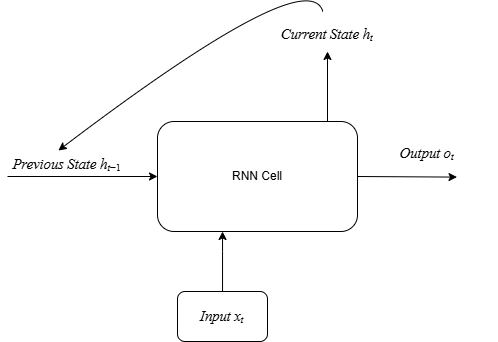
RNNs are the antithesis of this. By their very definition, they are sequential. To compute the hidden state for word t (h_t), you must have already computed the hidden state for word t-1 (h_{t-1}). There's no way around it. You cannot calculate the context for the word "cat" in "The cat sat on the mat" before you've calculated the context for "The".
This inherent dependency means you can't throw all the words of a sentence at the GPU at once and process them in parallel. The computation has to happen in a strict, linear order. In an age of massively parallel hardware, this was like trying to fill a swimming pool with a single garden hose. It was a fundamental mismatch between the algorithm's design and the hardware's capability, making the training of models on very large datasets incredibly slow and computationally expensive.
This bottleneck wasn't just an inconvenience; it was a hard limit on progress. To build bigger, more powerful models, the field needed a way to break free from this one-at-a-time processing. But the speed problem was only half of the story. The other, more insidious problem had to do with memory itself.
b. The Long-Term Memory Problem: Vanishing Gradients and Lost Context
Beyond the speed limitations, the sequential nature of RNNs creates a much deeper, more fundamental problem: they are terrible at remembering things for a long time.
Remember how an RNN works: it passes a "hidden state" or "context vector" from one time step to the next. This vector is supposed to be a summary of everything the model has seen so far. To update this summary, it's repeatedly multiplied by weight matrices at every single step.
Now, imagine a long and complex sentence like:
"In the first chapter of the book I was reading in France, a country renowned for its culinary traditions, the author describes a scene where the main character, a young girl, finds a lost cat..."
...and 100 words later, the sentence ends with:
"...and so she decided to name it Marie."
For the model to understand that "it" refers to the "cat," it needs to have carried the information about the "cat" all the way through 100 steps of processing. At each of those steps, the context vector is being transformed by matrix multiplications and passed through activation functions.
During training, the model learns by calculating an error at the end and sending a "gradient" signal backwards through the network to update the weights. In an RNN, this gradient has to flow backwards through every single time step. If the gradient signal is repeatedly multiplied by numbers smaller than 1, it shrinks exponentially until it becomes virtually zero it vanishes. If it's multiplied by numbers larger than 1, it can grow exponentially until it becomes unusable it explodes.
The "vanishing gradient problem" is the more common and notorious issue. It means that by the time the error signal from the word "it" travels all the way back to the word "cat," it has become so faint that it provides almost no information on how to adjust the weights. The network is effectively unable to learn dependencies between words that are far apart.
Its short-term memory is fine, but its long-term memory is practically non-existent. It forgets the beginning of the story by the time it reaches the end. This was the second, more profound wall that sequence modeling had hit.
We needed a new kind of architecture. One that didn't rely on a long, fragile chain of sequential operations. We needed a model where the path between any two words was direct and short, no matter how far apart they were in the sequence.
3. The Solution: Attention Is All You Need
The year is 2017. The world of NLP is dominated by recurrent architectures. Then, a team at Google Brain releases a paper with a bold, almost defiant title: "Attention Is All You Need." This paper didn't just propose an improvement; it proposed a revolution. It suggested throwing out recurrence entirely and building a new architecture based solely on a powerful mechanism called attention.
This new architecture was named The Transformer.
Let's start by looking at the model from a 10,000-foot view. In a task like machine translation, it acts as a single black box, taking a sentence in one language and outputting its translation in another.

Now, let's pop the hood on this black box. We see that, like many previous models, it has two main components: an encoding component and a decoding component.

The job of the encoding component is to read the entire input sentence (e.g., "Je suis étudiant") and build a rich, contextualized numerical representation of it. The job of the decoding component is to take that representation and, one word at a time, generate the translated output sentence (e.g., "I am a student").
So far, this looks familiar. But the real innovation is what's inside these components. Instead of a single encoder and decoder, the Transformer uses a stack of them the original paper used a stack of six.

The input sentence flows through the stack of encoders, with the output of each encoder becoming the input for the next. The final representation from the top encoder is then made available to every single decoder in the decoder stack.
But what are these encoders and decoders made of? This is where the core architectural pattern of the Transformer is revealed. Each encoder and decoder shares a similar internal structure.
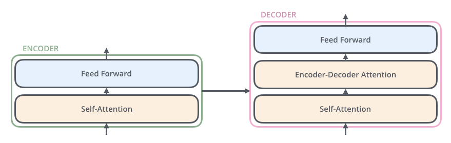
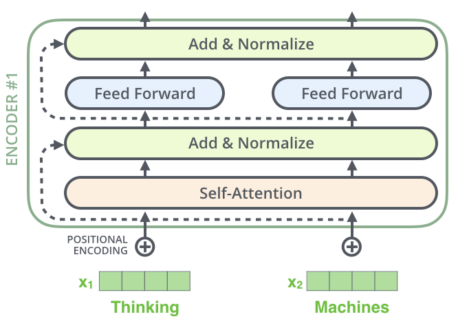
Let's look at a single encoder. It's composed of two main sub-layers:
A Self-Attention layer
A Feed-Forward Neural Network

This is the fundamental building block. The input to the encoder first flows through the self-attention layer. This is the layer that does the heavy lifting it's where each word in the input gets to look at all the other words to build a better understanding of itself in context. The output of this layer is then fed to a standard feed-forward neural network for further processing.
The decoder has a similar structure, but with a crucial third layer sandwiched in the middle: an Encoder-Decoder Attention layer. This layer allows the decoder to look back at the encoded input sentence and focus on the most relevant parts as it generates the output.
This architecture, built on stacks of attention and feed-forward layers, is the solution that breaks the "tyranny of the chain." It removes recurrence entirely, opening the door to massive parallelization. But how does this "Self-Attention" layer actually work? How does it allow words to "look at" each other? This brings us to the true heart of the Transformer.
4. The Strategy: A Conversation Between Words
We've arrived at the heart of the Transformer. We've thrown around the term "self-attention," but what does it actually mean? How can a model, without any recurrence, understand context?
Let's distill the concept with a powerful analogy.
a. From One-Way Memory to a Full-Blown Dialogue
Imagine an RNN as a person reading a book one word at a time. Their understanding of the story is based on the memory of the words they've just read. It's a one-way flow of information from the past to the present.
Our input sentence is:
”The animal didn't cross the street because it was too tired”
Now, imagine Self-Attention as a group of people in a meeting room, all trying to understand a single, complex sentence. Instead of speaking one by one, everyone gets to ask questions to everyone else, all at the same time.
The word "it" might shout, "Hey everyone, I'm a pronoun! Who in this sentence is the most likely thing I'm referring to?"
The word "animal" would raise its hand and say, "I'm a noun, and I was mentioned recently. It's probably me!"
The word "street" would stay quiet, recognizing it's an unlikely candidate.
Simultaneously, the word "tired" might ask, "I'm an adjective describing a state. Who is feeling this way?"
Again, "animal" would respond, "That's also likely me!"
After this instantaneous dialogue, each word in the room updates its own definition based on the answers it received. The word "it" is no longer just a generic pronoun; its representation is now blended with the representation of "animal" and "tired," creating a new, contextually rich vector.
This is the core idea of self-attention. It's a mechanism that allows every word in a sequence to directly interact with every other word, creating a "web of connections" instead of a linear "chain of memory." This process allows the model to bake the "understanding" of other relevant words into the one it's currently processing.

As you can see in that visualization, when the model is processing the word "it," its attention mechanism is quite literally "focusing on" or "listening to" the words "The" and "animal." It has learned that these words provide the most important context for understanding "it."
But how does this "dialogue" work mathematically? How does a word "ask a question" and how do other words "provide answers"? This is accomplished by giving each word three distinct personas.
b. The Three Personas of a Word: Query, Key, and Value
For this "dialogue" to happen, the Transformer architecture gives every single input vector (the embedding for each word) three different identities, or "personas." It creates these three vectors from each input word's vector by multiplying it by three separate, learned weight matrices (W_Q, W_K, W_V).
These new vectors are:
Query (q): The Query vector represents the word in its role as an interrogator. It's a vector that says, "Here's what I am, and here's the kind of information I am looking for to better understand myself."
Key (k): The Key vector represents the word in its role as a signpost or label. It's a vector that advertises, "This is the kind of information I contain." It's the "title" on the spine of a book, telling you what's inside.
Value (v): The Value vector represents the word's actual content or meaning. This is the core semantic information of the word.
The first step in any self-attention layer is to create these three vectors for every single word in the input sequence.

This diagram shows the process perfectly. The input embedding for "Thinking" (x1) is projected into its three personas: a query (q1), a key (k1), and a value (v1). The same happens for "Machines" (x2).
It's important to note that these new Q, K, and V vectors are typically smaller in dimension than the original embedding vector. This is an architectural choice that helps manage computational cost, especially when we introduce multiple attention heads.
Now that each word has a Query, a Key, and a Value, the dialogue can begin.
c. Calculating Relevance: The Query-Key Dot Product
How does the model figure out how much attention the word "it" should pay to the word "animal"? It does this by comparing the Query of "it" with the Key of "animal."
The mechanism for this comparison is simple and effective: the dot product.
The dot product is a fundamental operation in linear algebra that measures the similarity or alignment between two vectors.
If two vectors are pointing in a similar direction, their dot product will be a large positive number.
If they are unrelated (orthogonal), their dot product will be close to zero.
So, to calculate the attention score for a given word (e.g., "Thinking"), we take its Query vector (q1) and calculate the dot product with the Key vector of every word in the sentence, including itself.

In this example, when we're processing the word "Thinking" (position 1):
The first score is q1 · k1 = 112. This is the score of "Thinking" against itself, and it's usually the highest, as a word is most relevant to itself.
The second score is q1 · k2 = 96. This score measures how relevant the word "Machines" is to the word "Thinking."
This process is repeated for every word in the sequence. If we were processing "it," we would take its query, q_it, and compute the dot product with k_the, k_animal, k_didnt, and so on. The resulting high score for q_it · k_animal is the mathematical signal that these two words are highly relevant to each other.
These raw scores tell us the "relevance," but they're not yet clean, stable probabilities. That's the next step in our deep dive.
5. Deep Dive: The Mechanics of an Attention Head
We've established the high-level strategy: every word creates a Query, Key, and Value, and then uses its Query to score every other word's Key. This gives us a set of raw "relevance scores." Now, let's trace the precise mathematical journey these scores take to produce the final, context-rich output vector. This entire process happens within a single Attention Head.
a. Step 1: Creating the Q, K, and V Matrices
As we saw in the last section, the very first step is to take our input embeddings and project them into their Query, Key, and Value personas. While we looked at this on a word-by-word basis for intuition, in practice, this is done with a single, highly efficient matrix multiplication.
We start by packing the embedding vectors for all the words in our input sequence into a single input matrix, X. Then, we multiply this X matrix by the three learned weight matrices (W_Q, W_K, W_V) that we trained.
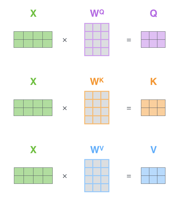
This single operation instantly gives us three new matrices:
Q (Query Matrix): Each row of this matrix is the Query vector for the corresponding word in the sentence.
K (Key Matrix): Each row is the Key vector for that word.
V (Value Matrix): Each row is the Value vector for that word.
Now we have all the ingredients we need for the attention calculation, neatly organized in matrix form.
b. Step 2 & 3: Calculating Scores and Scaling
The next step is to calculate the raw attention scores. As we discussed, this is done by taking the dot product of a word's Query with every other word's Key. In matrix form, this can be accomplished for all words simultaneously by multiplying the Query matrix Q by the transpose of the Key matrix Kᵀ.

This Q · Kᵀ operation results in a new "score" matrix. The value in row i and column j of this matrix is the dot product of the query from word i and the key from word j exactly the relevance score we wanted!
However, the authors of the "Attention Is All You Need" paper noticed a problem. As the dimensions of the Key vectors (d_k) get larger, the dot product values can grow very large in magnitude. When you feed very large numbers into a softmax function (our next step), it can push the gradients to be infinitesimally small, making the network very difficult to train.
To counteract this, they introduced a simple but crucial scaling step: they divide all the scores by the square root of the dimension of the key vectors, √d_k.

This scaling step helps to stabilize the gradients during training, making the whole process more robust.
c. Step 4: Softmax for Attention Weights
At this point, we have a matrix of scaled scores. The score in row i, column j represents how much attention word i should pay to word j. But these are just raw numbers. What we need is a clean distribution of "focus" that adds up to 100%.
This is a perfect job for the softmax function, which we've seen before in our Logistic Regression post.
We apply the softmax function to each row of our score matrix. The softmax function takes a vector of arbitrary real numbers and squashes it into a probability distribution. All the new values will be between 0 and 1, and they will all sum up to 1.

Let's revisit our "Thinking Machines" example. The scaled scores for the word "Thinking" against "Thinking" and "Machines" were 14 and 12.
softmax([14, 12]) = [0.88, 0.12]
This tells us that for the word "Thinking," the model has decided to place:
88% of its attention on itself ("Thinking").
12% of its attention on the word "Machines".
This resulting matrix is our attention weights matrix. It's a clear, quantifiable map of where each word in the sentence is focusing its attention.
d. Step 5 & 6: The Grand Finale - Multiplying by Value and Summing Up
We have the attention weights. We know how much to focus. But what are we focusing on? This is where the Value (V) vector finally comes into play.
Remember, the V vector holds the actual semantic meaning of each word. We now take the attention weights we just calculated and multiply them by the Value vectors.

The intuition is powerful:
Words we want to focus on (those with high attention weights, like 0.88) will have their Value vectors multiplied by a large number, preserving their meaning.
Words we want to ignore (those with low attention weights, like 0.001) will have their Value vectors multiplied by a tiny number, effectively drowning out their meaning.
This is done for each word in the sequence. To get the final output for the word "Thinking," we perform a weighted sum. We multiply each word's Value vector by the attention weight we calculated for "Thinking" and then sum up the results.
z1 = (0.88 * v1) + (0.12 * v2)

This final vector, z1, is the output of the self-attention layer for the word "Thinking". It is a new representation of "Thinking" that is context-aware. It is composed of 88% of the meaning of "Thinking" and 12% of the meaning of "Machines."
This entire, intricate dance can be condensed into a single, elegant formula for the entire sequence:

This single line of math encapsulates the entire process of creating Q, K, and V, scoring, scaling, applying softmax, and multiplying by V to get the final output matrix Z. Each row of Z is the new, contextually-aware vector for each word, ready to be passed up to the next layer in the Transformer.
6. The Beast with Many Heads: Multi-Head Attention
We've just walked through the entire, elegant process of a single self-attention head. It allows every word to look at every other word and create a new, context-rich representation. But the authors of the "Attention Is All You Need" paper found that a single attention head, while powerful, could still be limiting.
Think back to our "dialogue in a room" analogy. Having one self-attention calculation is like having the entire conversation dominated by one single topic. For example, when processing the sentence "The animal didn't cross the street because it was too tired," the word "it" might focus on "animal" to resolve its pronominal reference. But what if it also needs to understand the reason for the action? It might also benefit from focusing on "tired."
A single attention distribution for "it" might be a blend of focus on both "animal" and "tired," potentially diluting both signals. What if we could have multiple, parallel conversations happening at the same time, each focusing on a different aspect of the sentence?
This is the core idea behind Multi-Head Attention.
Instead of having just one set of Query, Key, and Value weight matrices (W_Q, W_K, W_V), the Transformer has multiple sets (the original paper used eight heads).

This diagram is key. Each attention head gets its own, independently learned set of weight matrices. This means that when the input X is projected, each head creates its own unique Q, K, and V matrices.
Think of this as giving our model multiple "representation subspaces."
Head 0 might learn to project the embeddings into a subspace where it can best calculate syntactic relationships (e.g., "it" refers to "The animal").
Head 1 might project them into a different subspace where it can track the relationship between actions and states (e.g., "cross" is related to "tired").
Head 2 might just be tracking which word is a verb, and so on.
Each head can learn to focus on a different aspect of the language, all in parallel.
The self-attention calculation we just detailed is then performed eight separate times, once for each head, using each head's unique Q, K, and V matrices.

This results not in a single output matrix Z, but in eight different Z matrices. Each of these Z matrices represents a different, context-aware "view" of the input sentence. Z0 might have encoded the pronoun relationships, while Z1 might have encoded the causal relationships.
This gives us an incredibly rich, multi-faceted representation of the input. But it also leaves us with a challenge: the next layer in our Transformer, the Feed-Forward Network, is expecting a single matrix, not eight. How do we resolve this?
So, each of our eight attention heads has done its work, producing its own unique output matrix (Z0, Z1, ..., Z7). We now have a wealth of information, but it's spread across eight different matrices. The Feed-Forward Network that follows is expecting a single matrix, where each row corresponds to a single word. We need a way to combine these eight outputs into one.
The solution is straightforward and effective:
Concatenate: We take the eight matrices and concatenate them together, end-to-end.
Project: This concatenated matrix is now very wide. To get it back to the original dimension that the model expects, we multiply it by one final, learned weight matrix, W_O. This matrix acts as a projection layer, taking the rich information from all eight heads and condensing it back into a single, unified output matrix Z.

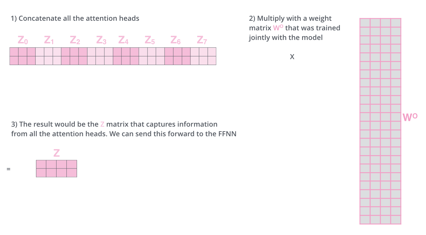
This final matrix Z is the output of our Multi-Head Attention layer. Each row of this matrix is a vector that contains information not just from one attention "dialogue," but from all eight parallel dialogues, each focused on a different aspect of the input.
Let's put it all together in one grand visual.

This single diagram beautifully summarizes the entire process:
The input sentence is embedded.
The embeddings are multiplied by eight different sets of W_Q, W_K, W_V weight matrices to create eight sets of Q, K, V matrices.
Self-attention is calculated in parallel for each head, producing eight Z matrices (Z0 to Z7).
These Z matrices are concatenated.
The concatenated matrix is multiplied by the final weight matrix W_O to produce the single output of the layer.
This entire block is then ready to be passed on to the Feed-Forward Network, and this completes one full "Encoder" layer.
7. Putting It All Together: The Full Transformer Architecture
We've spent the last few sections on an intense deep dive into the Multi-Head Attention mechanism. This is, without a doubt, the most important conceptual piece of the Transformer. Now that we've mastered it, we can zoom back out and quickly assemble the remaining components to see the full, end-to-end architecture in all its glory.

This diagram shows the complete model. Let's briefly touch on the final pieces of the puzzle.
a. The Encoder and Decoder Stacks
As we saw in our high-level overview, the Transformer isn't just one Encoder and one Decoder. It's a stack of them (the original paper used N=6). The input sentence flows up through the entire Encoder stack. The output of the final Encoder is a set of attention vectors, K and V, that represent a rich, contextualized understanding of the entire input sentence. This output is then fed into every single Decoder in the Decoder stack, allowing each decoder to focus on relevant parts of the input sentence while it generates the output.
b. Positional Encodings: The Missing Sense of Order
This is the crucial piece that allows a model without recurrence to understand word order. Before the input words are fed into the first encoder, a Positional Encoding vector is added to each word's embedding.
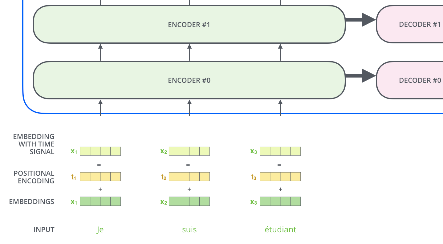
These are not random vectors. They are generated using a clever formula involving sine and cosine functions of different frequencies.

You don't need to memorize the formula. The key intuition is that these encodings create a unique "signal" or "fingerprint" for each position in the sequence. By adding this signal directly to the word embeddings, the model can learn to distinguish between "The cat chased the dog" and "The dog chased the cat" because the embeddings for "dog" and "cat" will be slightly different in each sentence based on their position. This allows the model to learn about the relative positioning of words during the attention calculation.

c. Residuals & Normalization: The Glue That Holds It All Together

Look closely at the full architecture diagram again. You'll notice that after every sub-layer (both Self-Attention and the Feed-Forward Network), there's an "Add & Norm" step. This represents two critical engineering tricks:
Residual Connections: The input to the sub-layer is added directly to the output of the sub-layer. This is a "skip connection" that allows the gradient to flow directly through the network during training, making it possible to build very deep stacks of encoders and decoders without the vanishing gradient problem we saw in RNNs.
Layer Normalization: After the residual connection, the output is normalized. This helps to stabilize the training process by keeping the values within a consistent range.
These two components are the essential "glue" that holds the deep architecture together and allows it to be trained effectively. And with that, we have assembled the entire Transformer, from input embedding to final output.
8. Going Deeper: Build Your Own Transformer in the Vizuara AI Lab!
We've journeyed through the entire Transformer architecture, from the high-level concept of parallel processing down to the intricate dance of Queries, Keys, and Values. We've seen the diagrams and unpacked the formulas. But to truly internalize how this web of attention works, there's no substitute for seeing the numbers crunch and flow yourself.
That's why we've built the next chapter of our learning series in the Vizuara AI Lab. This isn't just a code walkthrough; it's a hands-on environment where you become the computational engine of the Transformer. In our lab, you will:
Manually create Query, Key, and Value vectors from input embeddings.
Calculate attention scores step-by-step to see how the model learns relevance.
Visualize Multi-Head Attention, watching how different heads focus on different parts of a sentence.
Build a complete Encoder layer from the ground up, connecting all the components we've discussed.
Reading is knowledge. Calculating is understanding. Are you ready to master the architecture that powers modern AI?
9. Conclusion: The Dawn of a Parallel Universe
Our journey began at "The Wall of Sequential Processing," where the very nature of RNNs held the field of AI back. Their one-word-at-a-time approach was slow, inefficient, and forgetful over long distances. We saw how this "tyranny of the chain" created a fundamental bottleneck.
Then came the revolution: the Transformer. By discarding recurrence entirely and embracing the power of Self-Attention, the authors of "Attention Is All You Need" ushered in a new era. We've seen how this architecture allows every word to engage in a simultaneous dialogue with every other word, creating a rich, contextual understanding in parallel. We dove deep into the mechanics of Queries, Keys, and Values, and saw how multiple attention heads could work together to form a nuanced, multi-faceted view of language.
The shift from the sequential chain of RNNs to the parallel web of the Transformer was more than an incremental improvement; it was a complete paradigm shift. It unlocked the ability to train massive models on unprecedented amounts of data, paving the way for the Large Language Models like GPT, LLaMA, and DeepSeek that we know today. You now understand the core engine that drives the most advanced AI in the world.
10. References
This article is a conceptual deep dive inspired by the groundbreaking work of researchers and engineers in the AI community. For those wishing to explore the source material and related concepts further, we highly recommend the following papers and resources:
[1] Vaswani, A., Shazeer, N., et al. (2017). Attention Is All You Need. arXiv:1706.03762. (The original, seminal paper that introduced the Transformer.)
[2] Alammar, J. (2018). The Illustrated Transformer. (An excellent, highly-visual blog post that provides a fantastic intuition for the architecture.)
[3] Ferrer, J. (2024). How Transformers Work: A Detailed Exploration of Transformer Architecture. DataCamp. (A comprehensive tutorial on the Transformer architecture.)
[4] Amanatullah. (2023). Transformer Architecture explained. Medium. (A well-structured explanation of the Transformer's components.)
[5] Abideen, Z. (2023). Attention Is All You Need: The Core Idea of the Transformer. Medium. (A focused deep dive into the self-attention mechanism.)
Stay Connected
So.. that's all for today.
Follow me on LinkedIn and Substack for more such posts and recommendations, till then happy Learning. Bye👋