
Diffusion Model Visual Breakdown
How diffusion models turn noise into images.

This Blog Covers
Why earlier generators such as GANs and VAEs left room for a different approach
The diffusion idea: learn to reverse a noising process
The small set of equations needed to read a DDPM diagram
How U-Nets, timestep embeddings, and latent spaces make diffusion practical
How conditioning and transformer backbones shape modern image generation
1.0 Introduction
Image generation used to be easy to describe and hard to train. A generator would take a random vector and try to turn it into a realistic image. If the image looked wrong, the training signal had to explain what was wrong. That sounds reasonable until you remember how many ways an image can fail. The subject can be distorted, the texture can be weak, the pose can collapse, the background can look fake, or the image can be sharp but repetitive. A single image is not one decision. It is a large collection of decisions that need to agree.
Diffusion models became important because they change the shape of the problem. Instead of asking a neural network to create a full image in one shot, they ask it to solve a much smaller task many times: given a noisy image, predict how to remove a little of the noise. The same model repeats that correction from heavy noise to a clean image. This makes generation feel less like a leap and more like a guided recovery process.
This chapter starts with the older ideas because they explain why diffusion was such a useful turn. GANs showed that learned generators could make sharp, impressive images, but adversarial training could be fragile. VAEs showed that a model could learn a useful latent space, but samples often looked too smooth. Diffusion combines a different training target with a gradual sampling process. It is not free, since sampling can require many network calls, but the training signal is simple, stable, and visually powerful.
We will keep the math focused. You do not need a full derivation to understand why diffusion works. You need to know how clean images are mixed with Gaussian noise, why a timestep matters, what the denoiser predicts, and how repeated denoising turns a random sample into an image.
1.1 Why generative models needed another path
Before diffusion models became the standard tool for image generation, two families shaped most of the conversation: generative adversarial networks and variational autoencoders. They are worth covering first because diffusion did not replace an empty space. It solved pain points that became clear through years of work with older generators.
GANs were exciting because they could produce crisp images. The generator learned to map a random vector to an image, and a discriminator learned to judge whether an image came from the training set or from the generator. The generator improved by trying to fool the discriminator. This setup created a learned realism signal, which was much richer than a hand-written pixel loss.
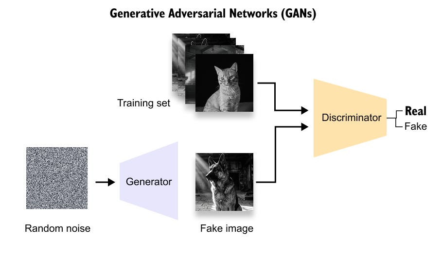
Figure 8.1. A basic GAN setup. The generator maps random noise to fake images. The discriminator receives both real training images and generated images, then predicts whether each input is real or fake. The generator improves by trying to fool the discriminator, so the training signal comes from a learned critic rather than from a fixed reconstruction loss.
As shown in Figure 8.1, a GAN is a two-network game. This game is the source of its strength and also the source of many practical problems. If the discriminator becomes too good too quickly, the generator may get weak gradients. If the generator finds a small set of outputs that fool the discriminator, it can repeat those outputs and lose diversity. This failure is often called mode collapse. The samples may be sharp, but the training process can feel like balancing two moving targets.
This contrast is useful throughout the chapter. In a GAN, the generator learns from the discriminator’s current opinion. In a diffusion model, the target for a training example is the exact noise that was added by the training code. That target is not another network’s opinion. It is a known value. This does not make diffusion magically easy, but it removes the adversarial game from the core training loop.
VAEs took a different route. A variational autoencoder learns to encode an image into a latent distribution and decode a latent sample back into an image. This gives the model a compressed internal space, which is a useful idea for generation and editing. The tradeoff is that VAE samples and reconstructions often look smoother than GAN samples, especially when the decoder is trained with losses that reward average-looking reconstructions.
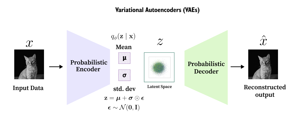
Figure 8.2. A variational autoencoder. The encoder maps input data to a latent distribution, a latent sample is drawn, and the decoder reconstructs the output. VAEs are important for this chapter because modern latent diffusion systems borrow the idea of working in a compressed representation, then use diffusion to model that latent space more powerfully.
As shown in Figure 8.2, the part of the VAE story that survived strongly into modern systems is compression. A good latent representation can keep the meaningful structure of an image while using far fewer values than the original pixels. Diffusion models later used this idea to reduce cost. Instead of running the denoising model directly on every pixel, latent diffusion runs it on a smaller latent tensor and decodes the result at the end.
Older generators taught the field two lessons. First, sharp images matter, and a model needs a strong learned signal for realism. Second, the representation matters, because pixel space is expensive. Diffusion uses both lessons but changes the training problem. It turns image generation into the task of learning how to remove noise at many levels of corruption.
That change sounds modest, but it is a major shift in supervision. A GAN has to learn from a moving discriminator. A VAE has to balance reconstruction quality against a regularized latent space. A diffusion model can create its own training pairs. The input is a noisy version of a real image, and the target is the noise that the training code added. This gives the model many cleanly defined tasks from each training image.
It also changes how we should think about creativity in the model. The denoiser is not storing a library of clean images and retrieving one during sampling. It learns the local direction from “less likely under the data” toward “more likely under the data” at many noise levels. When sampling begins from random noise, those local directions are applied again and again. The final image is the result of the full path, not a single lookup.
This is the motivation for the rest of the chapter. Diffusion is useful because it breaks a hard one-shot generation problem into a sequence of denoising problems. The cost is that sampling has to run the model repeatedly. The benefit is that each training example has a simple, known target, and this makes the method easier to scale than adversarial training in many settings.
1.2 The Diffusion Idea
The central idea of diffusion is simple: take real data, slowly corrupt it into noise, and train a model to reverse that corruption. During training, the forward corruption process is not learned. We define it. During generation, the reverse process is learned. The model starts from noise and repeatedly takes small steps toward a cleaner sample.
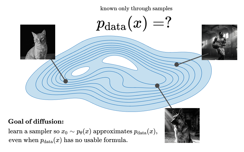
Figure 8.3. The goal of diffusion modeling. The true image distribution Pdata(x) is known only through examples, not through a neat formula. A diffusion model learns a sampler that starts from a simple base distribution and gradually moves toward regions that look like the training data.
As shown in Figure 8.3, the problem can be read from a distribution point of view. The training images are samples from a complicated image distribution. We do not know the full distribution, and we cannot directly sample new images from it. What we can sample from easily is Gaussian noise. Diffusion connects these two worlds by defining a path from data to noise, then learning how to travel back.
This path is easier to understand if you imagine a clean image being damaged step by step. At first, the subject is still visible. Later, only broad structure remains. At the end, the image is essentially noise. Because we control this damaging process, we can create unlimited supervised training examples from every image: pick a timestep, add the right amount of noise, and ask the model to predict the noise that was added.
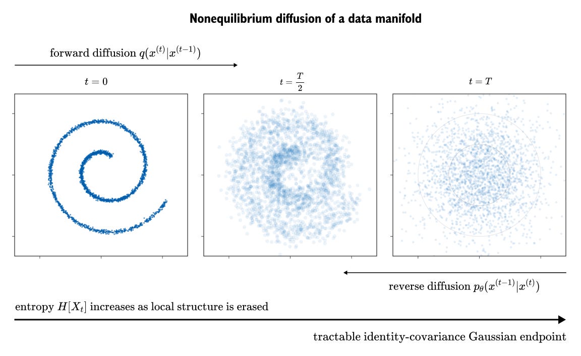
Figure 8.4. A data manifold being diffused into a simple noise distribution. At t=0, the samples lie on a structured spiral. As the forward process adds noise, the structure spreads out and eventually becomes close to an isotropic Gaussian. The reverse process learns to move in the opposite direction, from the easy endpoint back toward the structured data.
The toy dataset in Figure 8.4 is two dimensional, but the picture is the same for images. The structured data starts on a thin, meaningful shape. Noise gradually washes that structure out until the final distribution is simple. The reverse model learns how to move a sample from the noisy cloud back toward the kind of structure seen in the training data.
This is why diffusion can feel backward at first. We spend training time destroying images. The point is that controlled destruction gives us a clean learning signal. If the training code added a particular noise pattern, the network can be trained to recover that pattern. Generation then uses the trained network in the opposite direction.
NOTE
Diffusion does not mean that the first noise sample secretly contains the final image. The initial noise is random. The trained denoiser and the condition, such as a text prompt, guide the sample through many small corrections until it becomes image-like.
1.3 Why the endpoint is Gaussian noise
Every generator needs a starting point. If the starting point is already complicated, sampling is already hard. Diffusion models usually start from a standard Gaussian distribution,
This distribution is easy to sample from, easy to reason about, and flexible enough to act as a neutral blank canvas. It does not prefer faces, dogs, product photos, outdoor scenes, or any other category. The structure comes from the learned reverse process.
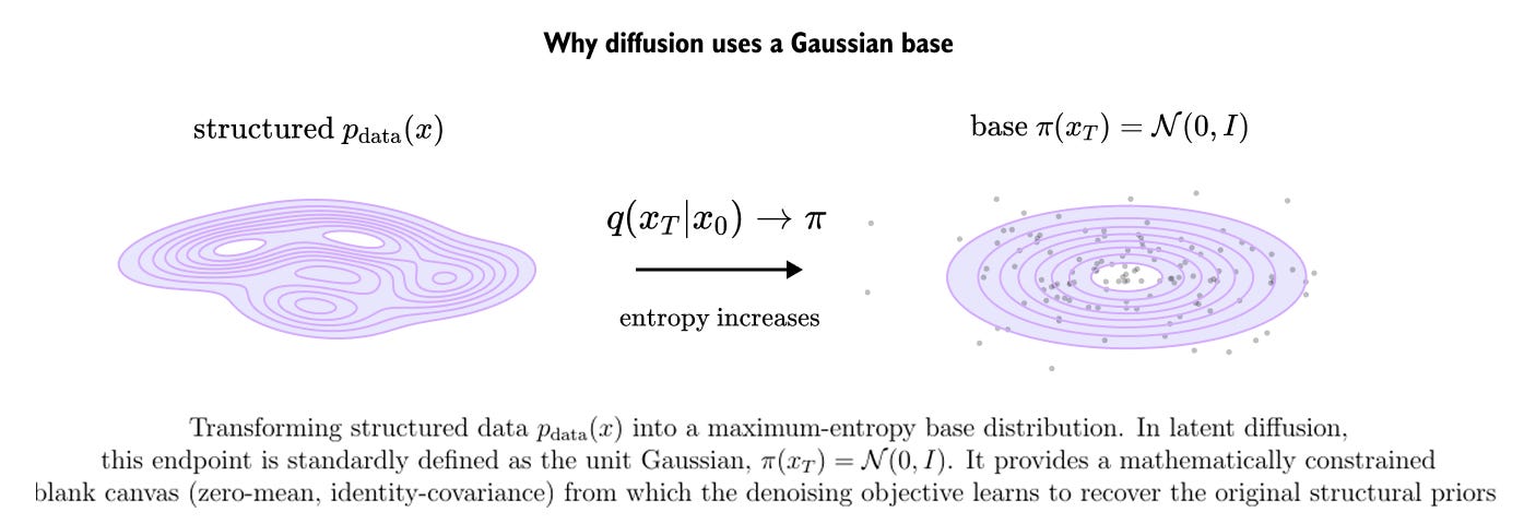
Figure 8.5. Why diffusion models use a Gaussian base. The structured data distribution is hard to sample from directly, but a maximum entropy Gaussian endpoint is easy to sample from. The forward process transforms structured data into that endpoint, and the reverse process learns how to undo the transformation.
The distribution-level reason is shown in Figure 8.5. A simple Gaussian endpoint lets us begin generation from something we can produce on demand. If we can learn a reliable reverse path from this endpoint to the data distribution, then sampling becomes possible even though the original image distribution is too complex to write down.
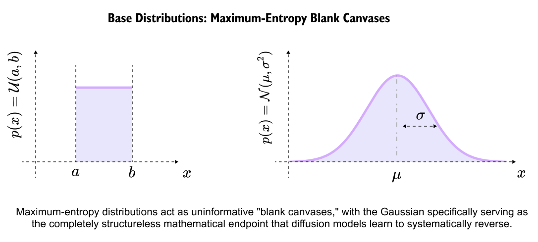
Figure 8.6. Base distributions as blank canvases. A uniform distribution and a Gaussian distribution are both high entropy choices, but Gaussian noise is especially convenient for diffusion because repeated additive Gaussian noise stays Gaussian and leads to a tractable endpoint for the forward process.
Possible blank canvases are compared in Figure 8.6. In practice, Gaussian noise is convenient because adding independent Gaussian noise repeatedly behaves cleanly. The endpoint remains mathematically manageable, and the training code can directly sample noisy versions of an image at any timestep. This is a practical choice, not a mystical one.
The important point is that the base distribution is simple on purpose. The model should not need a hand-designed image prior at the start. It should learn image structure from data and from the conditioning information.
1.4 The Forward Process
The forward process is the noising process we define. At each timestep, the clean image keeps some of its signal and receives some new Gaussian noise. The standard notation uses
for the amount of new noise at step
The matching signal retention is
The cumulative signal after many steps is
You can read
as “how much of the original image is still present after step
Early in the chain, this value is close to 1. Late in the chain, it is close to 0.
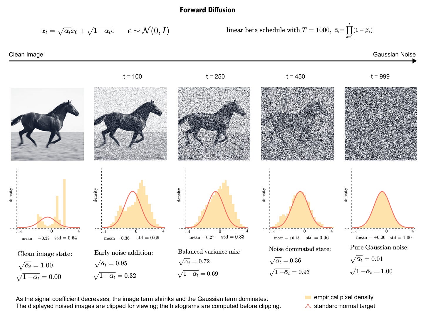
Figure 8.7. Forward diffusion on an image. The clean horse image is progressively corrupted with Gaussian noise. The distributional view below it shows the same change in coefficients: the signal coefficient decreases, the noise coefficient increases, and the noisy sample becomes less tied to the original image.
The sequence in Figure 8.7 is one of the most important ideas in the chapter. The model is not trained only on clean images and pure noise. It sees many intermediate states. Some examples are barely corrupted. Some are heavily corrupted. This gives the network a curriculum of denoising problems across the whole path from data to noise.
The math you actually need
The forward process can be sampled in one step:
\(\mathbf{x}_t = \sqrt{\bar{\alpha}_t}\mathbf{x}_0 + \sqrt{1-\bar{\alpha}_t}\boldsymbol{\epsilon}, \qquad \boldsymbol{\epsilon} \sim \mathcal{N}(\mathbf{0}, \mathbf{I}).\)This equation says that a noisy image is a weighted mixture of the clean image
\(\mathbf{x}_0\)and pureGaussian noise
\(\boldsymbol{\epsilon}\)The value
\(\bar{\alpha}_t\)Controls the signal part, and
\(1-\bar{\alpha}_t\)controls the noise part.
This equation is worth remembering because it explains how training examples are made. We do not need to simulate every previous step to get Xt We can sample a random timestep t, sample a random noise tensor
, and mix the clean image with that noise using the formula above. That single line is the workhorse behind DDPM-style training.
The square roots in the equation are there because the formula is balancing variance, not ordinary image brightness. You do not need to derive this to use the equation. A useful reading is that
scales the clean image and
scales the noise. When t is small, the clean coefficient is large and the noise coefficient is small. When t is large, the clean coefficient shrinks and the noise coefficient dominates.
This also explains why a noisy training sample is still tied to one clean image. At early timesteps, the noisy sample clearly resembles its source. At later timesteps, the source becomes harder to see, but the training code still knows exactly which clean image and which noise tensor created it. The denoiser receives the noisy sample and the timestep, then learns how much of what it sees should be treated as removable noise.
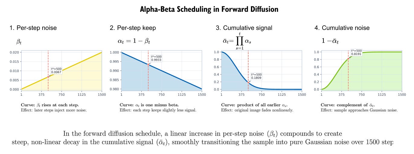
Figure 8.8. Alpha-beta scheduling in forward diffusion. The beta schedule controls the new noise injected at each step. The alpha values track per-step signal retention, while the cumulative product
tracks how much of the original image remains after many steps.
The curves in Figure 8.8 explain the schedule.
decides how aggressively noise is added at a particular step.
is the part of the signal kept at that step.
is the accumulated signal retention after many steps. A good schedule makes the denoising tasks neither too easy nor too destructive. If the process destroys structure too quickly, the network sees many examples that are almost pure noise.
If it destroys structure too slowly, the sampling process wastes steps making tiny changes.
Modern systems may express the schedule through sigmas, log signal-to-noise ratios, or continuous time variables, but the beginner intuition is the same. A schedule controls how the problem changes as the sample moves from clean data to noise and back.
1.5 What the denoiser learns
The denoiser is the learned part of the system. It receives a noisy sample
the timestep t and often a condition c.
The condition could be a class label, a text prompt, a mask, an edge map, a depth map, a low resolution image, or another signal. In the basic noise-prediction view, the network outputs
which is its estimate of the noise that was used to create
The training target is known because the training code sampled the noise. That gives a simple supervised loss:
This is not the full probabilistic derivation, but it is the equation that explains the practical training loop. Add known noise, ask the network to predict that noise, and update the network when it is wrong.
The loss is simple, but the task is rich. At low noise levels, predicting the noise can mean finding small corruptions around edges and textures. At high noise levels, predicting the noise is tied to understanding which broad structures are plausible under the data and condition. The same loss therefore teaches both local cleanup and global structure, depending on which timestep was sampled.
This is one reason diffusion training is often easier to reason about than GAN training. The network is given a direct regression target. If the prediction is wrong, the loss says so in a straightforward way. The model may still be large, the data may still be messy, and the sampler may still require careful tuning, but the basic training signal is stable.
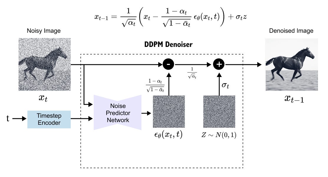
Figure 8.9. A DDPM denoising step. The noisy image Xt and timestep t enter the denoiser.
The network predicts the noise component
, and that prediction is used to compute the next, slightly cleaner sample
Generation repeats this step many times.
The denoising step in Figure 8.9 shows why diffusion sampling is iterative. The denoiser is not asked to jump straight from noise to the final image. It is asked to make one correction for the current noise level. When those corrections are repeated across a schedule, structure emerges gradually.
Predicting noise is a good first mental model because the target is exact. Some modern models predict the clean sample, a velocity target, or a flow direction instead. These variants matter in advanced systems, but they keep the same basic teaching idea: the model learns a direction that moves a noisy sample toward the data distribution.
The timestep is essential. A sample at a low noise level should be treated differently from a sample at a high noise level. At low noise, the model should refine edges and small details. At high noise, it must infer broad structure from weak evidence and from the condition. Without timestep information, the same network would not know which denoising problem it is solving.
It is also useful to separate the denoiser from the sampler. The denoiser predicts a target from the current noisy state. The sampler decides how to use that prediction to move to the next state. Two systems can use the same trained denoiser with different samplers and produce different speed-quality tradeoffs. A slow sampler may take many careful steps. A fast sampler tries to take fewer, larger steps without drifting away from the learned path.
This is why diffusion research often talks about both models and samplers. The model learns the direction. The sampler chooses the route. For a beginner, DDPM sampling is the easiest route to understand because it follows the chain step by step. Faster samplers keep the same goal but take a more efficient path through the noise levels.
1.6 Giving the network a sense of time
A timestep such as t=427 is just a number. Neural networks usually work better when important scalar values are expanded into richer representations. Diffusion models commonly use sinusoidal timestep embeddings, which turn a scalar timestep into a vector containing sine and cosine features at several frequencies.
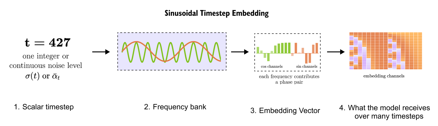
Figure 8.10: Sinusoidal timestep embedding. A scalar timestep, such as t=427, is converted into a vector using sinusoidal functions at multiple frequencies. This vector enters the denoising network so the same network can change its behavior at different noise levels.
As shown in Figure 8.10, the embedding gives the model a richer handle on time. Nearby timesteps produce related vectors, and distant timesteps produce different vectors. This is similar in spirit to positional embeddings in transformers, where position is turned into a vector that the model can use.
In a U-Net denoiser, the timestep embedding is usually injected into residual blocks. In a diffusion transformer, it may modulate normalization layers or block activations. The exact plumbing changes across architectures, but the purpose stays the same. The denoiser must know the current noise level before it can decide how aggressive its correction should be.
1.7 Why U-Nets Became The Classic Denoiser
For image diffusion, the classic denoising network is a U-Net. This is a practical match for the task. Denoising needs global context, because the model must understand what the image might contain. It also needs local precision, because the final output depends on edges, textures, alignment, and small spatial details.
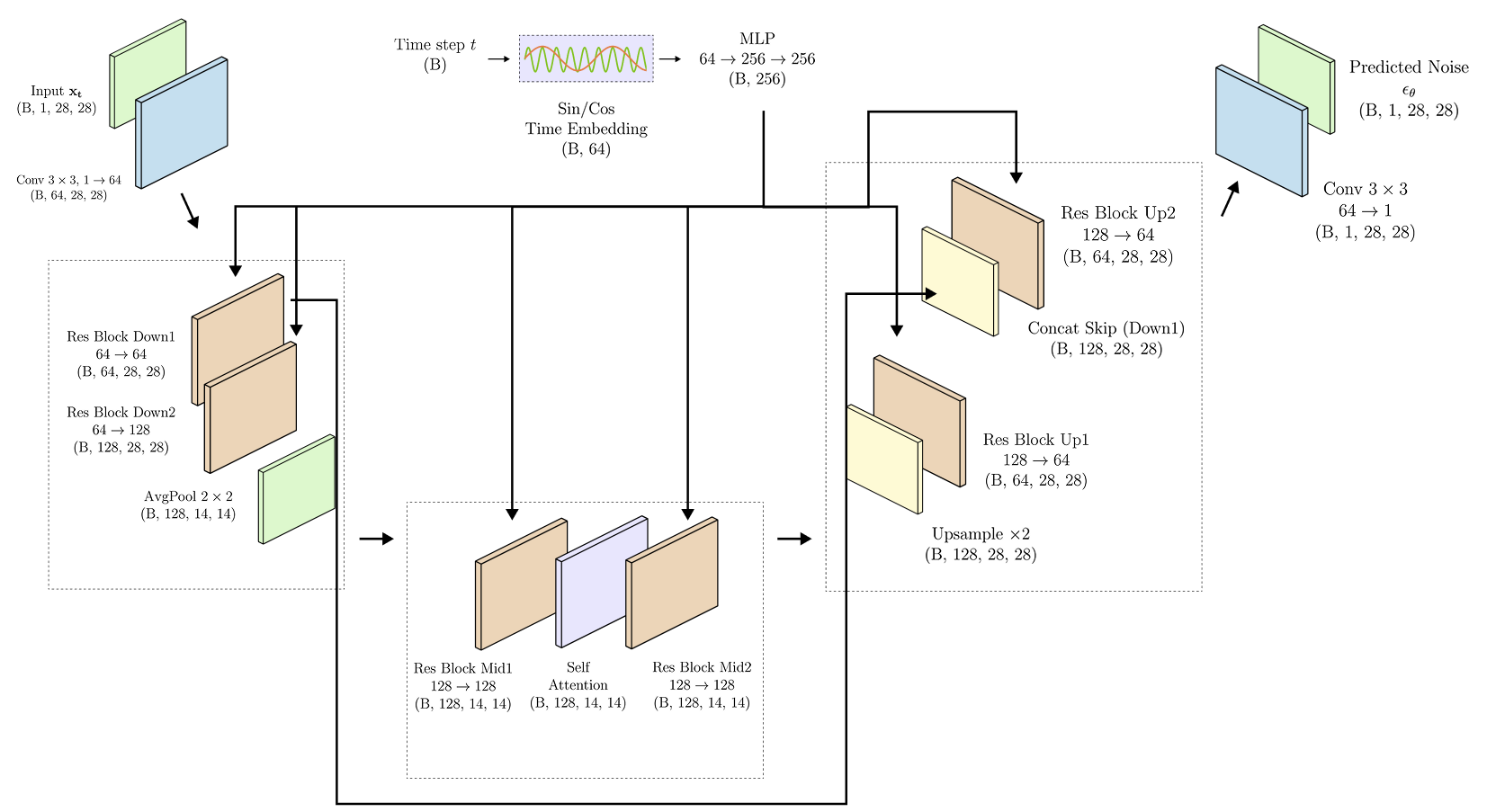
Figure 8.11. A U-Net denoiser for diffusion. The noisy image enters on the left. Down blocks reduce spatial resolution while increasing feature channels, middle blocks process a compact representation, and up blocks reconstruct a denoised output. Skip connections preserve fine spatial information that would otherwise be lost during downsampling.
The U shape in Figure 8.11 explains how the network handles both context and detail. The encoder path downsamples the image and builds wider feature maps. The decoder path upsamples back to the original resolution. Skip connections carry high resolution features from the encoder to the matching decoder stages. This lets the model use large-scale context without throwing away the precise spatial information needed for reconstruction.
This architecture fits the changing nature of diffusion. At high noise levels, the model needs broad semantic guesses: what object might be present, where the main shape might sit, and which condition should guide the composition. At low noise levels, it needs smaller corrections: sharper boundaries, smoother texture, and consistent local detail. The U-Net naturally supports both kinds of work. Attention layers are often added at selected resolutions so distant parts of the image can influence each other.
The denoiser can be written as
where c is optional conditioning information. If there is no c, the model is unconditional. If c is a class label, the model is class conditional. If c is a text embedding, the model becomes a text-to-image model. This notation is compact, but it captures a major design point: most modern diffusion systems differ in what they use as conditioning and how they inject it into the denoiser.
1.8 Latent Diffusion
Pixel-space diffusion is conceptually clean, but high resolution images are expensive.
A 512 X 512 RGB image has
values. A large denoising network may need to process that representation many times for a single sample. The cost grows quickly as resolution increases.
Latent diffusion reduces this cost by adding an autoencoder around the diffusion model. The encoder compresses an image into a smaller latent tensor. The diffusion model performs denoising in that latent space. The decoder turns the final denoised latent back into pixels. This is one of the main reasons high resolution text-to-image generation became practical on widely available hardware.
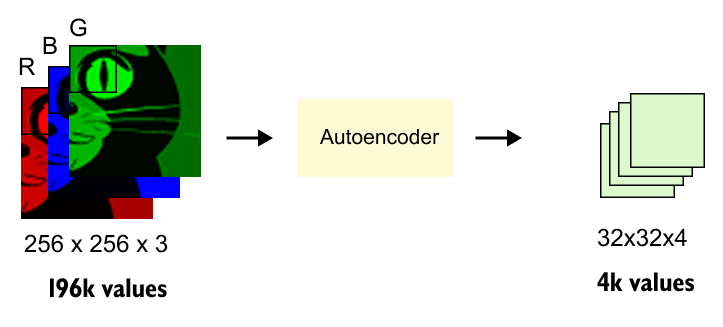
Figure 8.12. Image compression before diffusion. A 256x256x3 RGB image contains about 196k values. The autoencoder maps it to a 32x32x4 latent tensor with about 4k values. Denoising in this compressed space is far cheaper than denoising in pixel space.
The cost argument in Figure 8.12 is visible in the tensor sizes. The latent tensor is much smaller, but it can still preserve the information the decoder needs for a convincing image. The diffusion model no longer spends all its capacity modeling raw pixels. It works on a compressed space that is closer to perceptual structure.
There is a tradeoff. If the autoencoder compresses too hard, small text, fine geometry, faces, and repeated patterns may suffer. If it compresses too little, the diffusion model becomes expensive again. Latent diffusion is the practical compromise: keep enough visual information for good decoding, but reduce the denoising workload enough to make training and sampling feasible.
1.9 Conditioning: Making the Model Listen
Unconditional diffusion asks the model to generate something from the training distribution. Conditional diffusion asks it to generate something that matches an input. That input can be a label, a prompt, a low resolution image, a mask, an edge map, a depth map, a segmentation map, a pose skeleton, or another image. The denoising task is still the same, but the model receives extra information about where the sample should go.
Text-to-image systems usually encode the prompt with a text encoder and pass the resulting embeddings into the denoising network. U-Net systems often use cross-attention, where image features attend to text embeddings. The image features can then use words and phrases from the prompt as context while denoising. This is why prompt following is part architecture, part text encoder, part data, and part sampler behavior.
Cross-attention is easier to understand if you think of the noisy image features as asking for context. A feature at one spatial location may need to know which prompt tokens are relevant to that region. The attention operation gives the model a learned way to connect image features with language features. This does not guarantee perfect prompt following, but it gives the denoiser a path for using text during every denoising step.
Classifier-free guidance is a common way to make the condition stronger during sampling. During training, the model sometimes sees the condition and sometimes sees an empty condition. During sampling, we compare the conditional and unconditional predictions:
The guidance scale
controls how strongly the sample is pushed toward the condition. Low guidance leaves more freedom but may ignore parts of the prompt. High guidance follows the prompt more strongly but can reduce variety or create artifacts. It is a steering knob, not a pure quality knob.
Negative prompts and empty conditions fit naturally into this same idea. They change the direction of the guidance signal by telling the model what to move away from, what to ignore, or what should receive less weight. In practice, guidance works best when the prompt and negative prompt are treated as steering signals rather than as exact instructions. The model still generates through denoising, and the denoising path can only use patterns it learned during training.
Text is flexible, but it is not precise. If a user needs a subject to follow a pose, edge map, depth layout, or segmentation mask, text alone is usually too vague. Spatial control methods add structured signals to the denoising process. The common idea is to preserve the generative ability of a pretrained model while adding a trainable path that tells it how to use control inputs. This is why modern diffusion tools can follow sketches, poses, depth maps, masks, and other layouts.
1.10 Diffusion Transformers
The early image diffusion systems mostly used U-Nets. More recent systems increasingly use transformer backbones. The reason is familiar from other areas of deep learning: transformers scale well, process data as tokens, and allow long-range interactions through attention. In image diffusion, this usually happens in latent space. The model patchifies the latent tensor, turns patches into tokens, injects timestep and conditioning information, and predicts a denoising target.
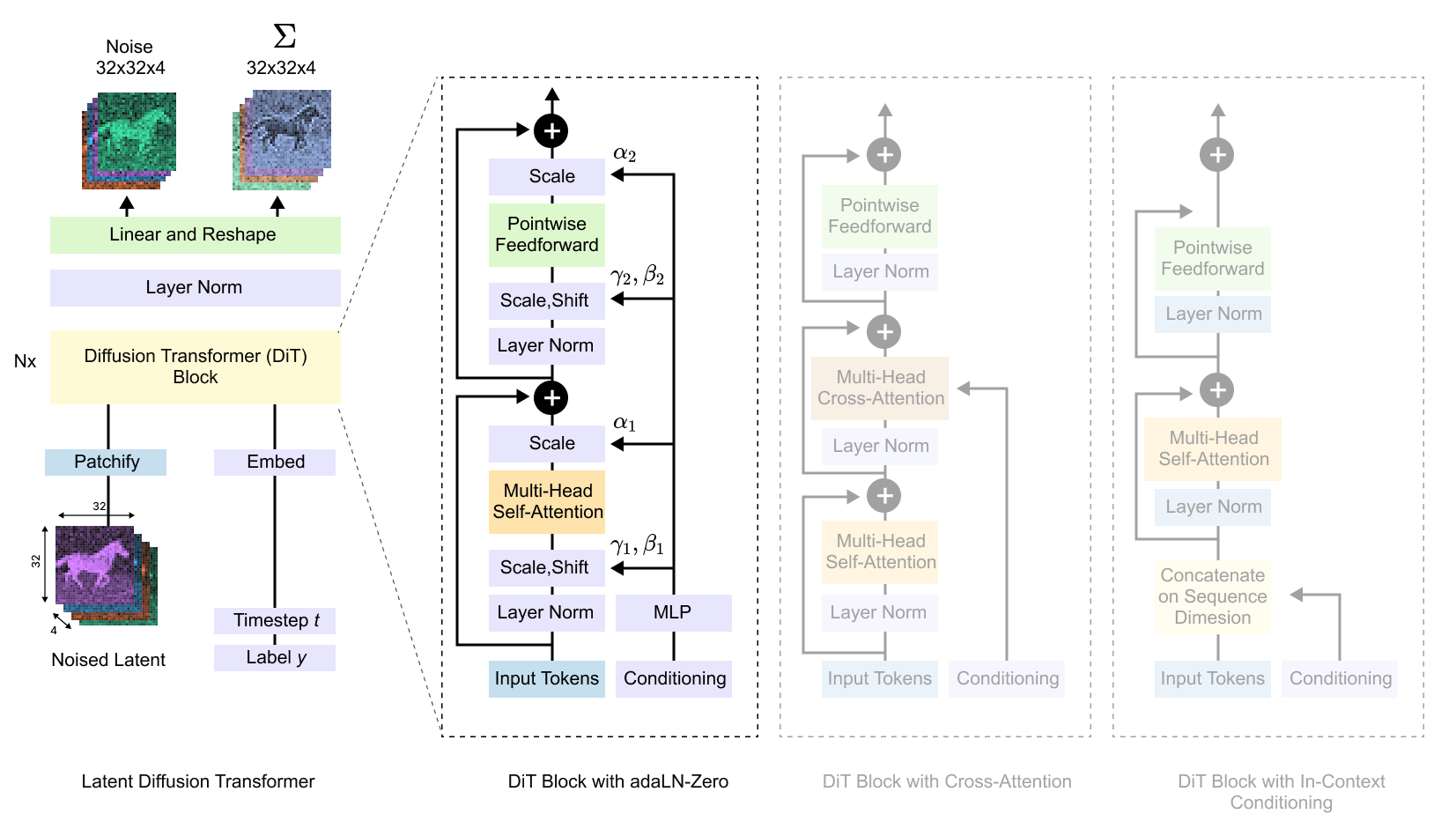
Figure 8.13. A diffusion transformer architecture. The noisy latent is split into patches and projected into tokens. Timestep and class-conditioning information modulate transformer blocks, and the output tokens are reshaped back into a latent prediction. This replaces the U-Net denoiser with a transformer denoiser.
The architecture in Figure 8.13 shows the shift from spatial feature maps to token processing. The denoising objective has not disappeared. The network backbone has changed. A diffusion transformer treats patches of the latent as tokens and uses attention to let those tokens interact.
If a latent tensor has height Hz width Wz and patch size p the number of patch tokens is roughly
Smaller patches preserve more spatial detail but increase attention cost. Larger patches are cheaper but coarser. This tradeoff is one reason diffusion transformer design often talks about patch size, token count, and compute together.
The transformer view is attractive because it gives the model a uniform way to mix information across the image. A token can attend to distant tokens without needing many convolutional layers between them. This can help with global layout, prompt alignment, and relationships between far apart regions. The price is attention cost, which grows quickly as the number of tokens increases.
Latent space helps again here. Patchifying a raw pixel image would create too many tokens for large models. Patchifying a compressed latent tensor is much more manageable. This is why diffusion transformers and latent diffusion fit together so naturally: the autoencoder reduces the spatial burden, and the transformer spends its compute on token interactions in the smaller space.
The next three examples connect the core ideas from this chapter to current text-to-image architectures. PixArt-alpha, MM-DiT, and Stable Diffusion 3 include many engineering details, but the useful lens here is architectural: how latent patches become tokens, how text enters the denoiser, how image and language streams interact, and how these pieces form a complete generation stack.
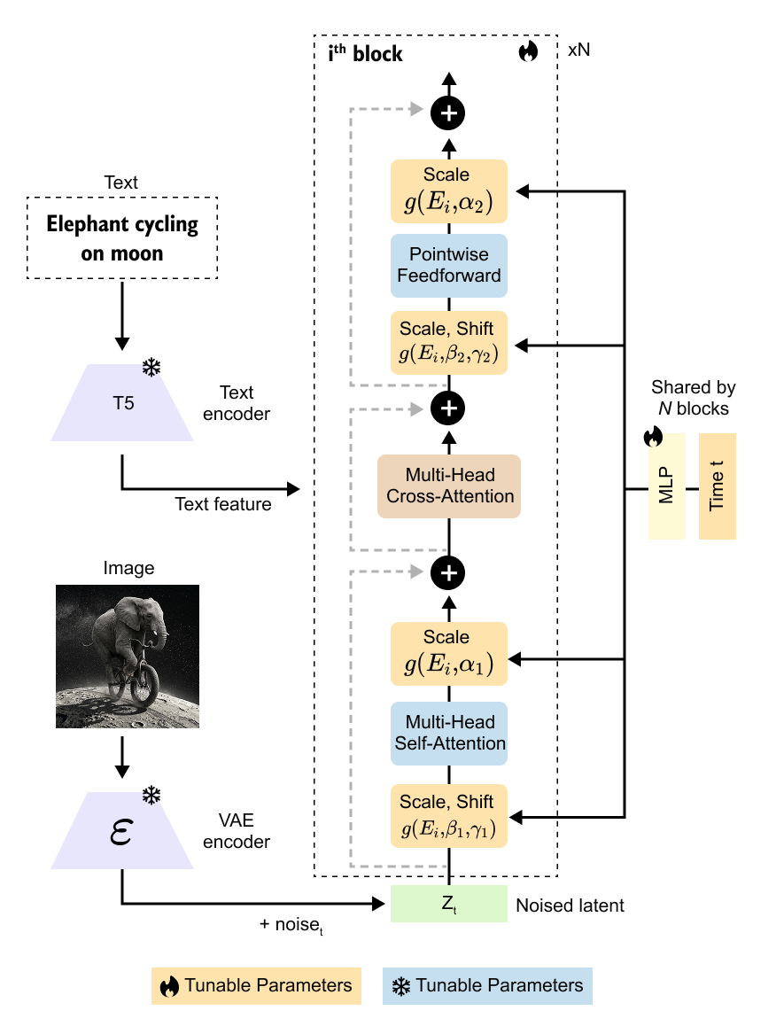
Figure 8.14. PixArt-alpha style text-to-image diffusion transformer. Text embeddings condition the denoising transformer, and the model operates on image latent tokens. The architecture emphasizes efficient transformer conditioning rather than a U-Net backbone.
The text-conditioning path is explicit in Figure 8.14. Text embeddings are not added at the end of generation. They influence the denoising computation inside the model. This is why a text-to-image system is more than an image generator with captions attached. The language representation shapes the denoising trajectory step by step.
Multimodal diffusion transformers go further by treating text tokens and image tokens more symmetrically. Instead of using text only as an external condition, the architecture can let text and image streams exchange information through joint attention. This gives the model a direct path for aligning language with visual structure.
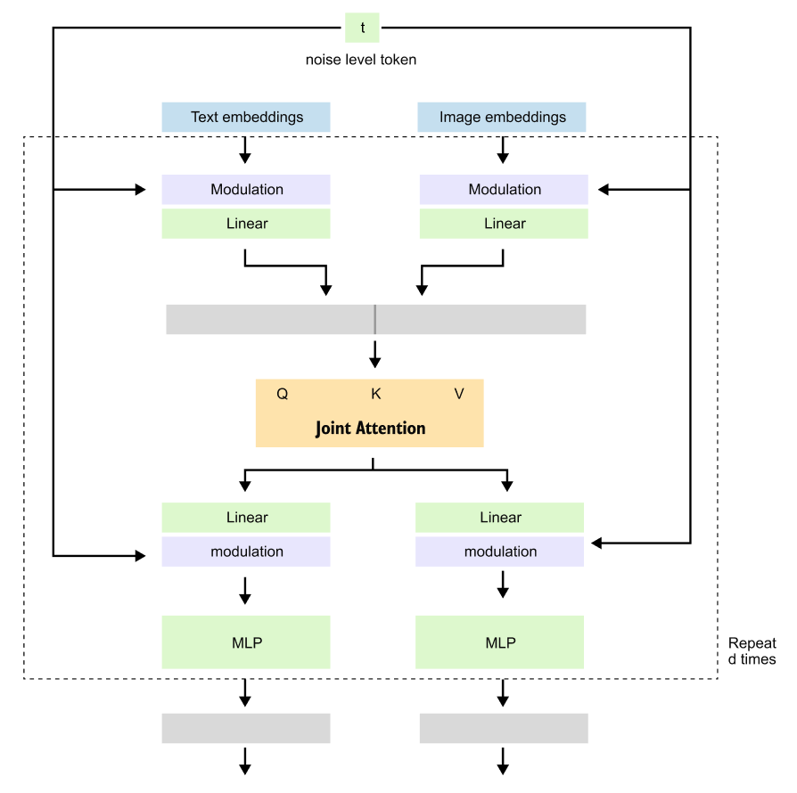
Figure 8.15. A multimodal diffusion transformer block. Text embeddings and image embeddings are processed as separate streams with modulation and MLP layers, while joint attention allows information to flow between the modalities. This design is used in the Stable Diffusion 3 family.
The block-level idea in Figure 8.15 is to process image and text streams separately while still connecting them through attention. Image and text tokens each have their own transformations, but attention connects them. The result is a denoising block that can update image information while checking it against language information.
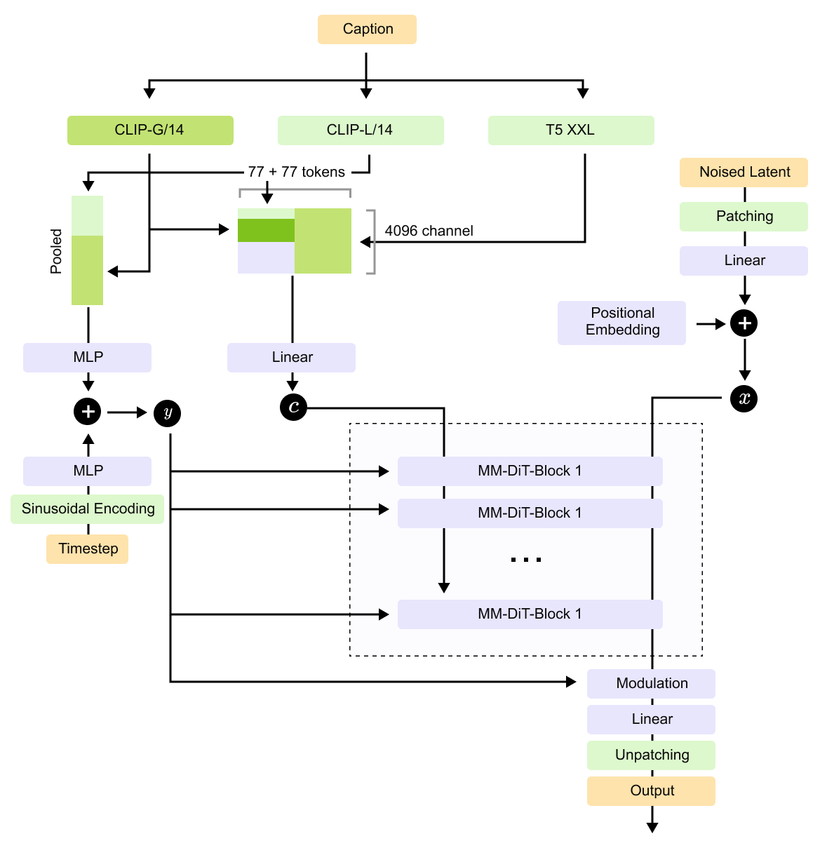
Figure 8.16. A Stable Diffusion 3 style architecture. Multiple text encoders produce conditioning signals, image latents are patchified, timestep information is embedded, and a stack of MM-DiT blocks performs the denoising computation before the output is unpatchified and decoded.
The full system in Figure 8.16 puts the pieces together. Text encoders produce conditioning signals, the image latent becomes a token sequence, timestep information tells the model where it is in the sampling path, and MM-DiT blocks perform the denoising computation. Stable Diffusion 3 style systems also use rectified-flow ideas, which you can think of at this level as another way to learn a path from noise to data.
The direction of modern image generation is clear even if the exact architecture keeps changing. Strong systems combine latent-space generation, powerful text encoders, transformer backbones, guidance, and carefully designed sampling paths. The diffusion idea remains the same: learn how to move from a simple noisy starting point toward a structured data sample.
1.11 Putting the pieces together
It helps to reduce the full pipeline to two stories: training and sampling. During training, we take a clean example, optionally encode it into a latent, choose a timestep, sample Gaussian noise, and mix the clean representation with that noise. The denoiser receives the noisy representation, the timestep, and any condition. It learns to predict the chosen target, often the noise itself. The target can differ across formulations, but the pattern is steady: corrupt a real example in a known way, then train a model to reverse that corruption.
During sampling, the direction flips. We start from random Gaussian noise. The denoiser predicts how to move one step toward a cleaner sample. The sampler applies that update and moves to a lower noise level. The process repeats until the final representation is clean enough to decode or display. If the model works in latent space, the last latent is passed through the decoder to produce pixels.
This explains both the strength and the cost of diffusion. The strength comes from many small, guided corrections. The cost comes from making many network calls. Faster samplers, distillation, consistency-style models, and flow-based formulations all try to reduce this cost while keeping the quality benefits of iterative generation.
Several design choices decide how a diffusion system behaves. The noise schedule controls which denoising tasks the model sees. The prediction target controls what the network learns to output. The backbone controls how spatial and semantic information move through the model. The conditioning path controls whether prompts, masks, depth maps, or other inputs are followed. The sampler controls the speed, quality, and amount of randomness during generation. The autoencoder controls how much information is available in latent space.
This is why two models can both be called diffusion models and still feel very different in use. They may share the same high-level path from noise to data, but use different schedules, denoisers, latent spaces, conditioning methods, and samplers.
1.12 Common Misconceptions
One common misunderstanding is that the model memorizes a reverse path for each training image. It does not. During training, the same clean image can be paired with many timesteps and many noise samples. The denoiser learns a general rule for moving noisy samples toward likely data, not a stored path back to one image.
Another misunderstanding is that the noise contains the image. The initial noise is just a random sample. The learned denoising function, the condition, and the sampler determine how that random sample turns into an image. Changing the random seed changes the starting point and often changes the final composition.
Prompt following is also easy to overestimate. A text-to-image model is not searching a database of captioned images. The prompt is encoded into vectors that condition the denoising process. The model has learned statistical relationships between text and image structure from data. This is why it can combine ideas in useful ways and also why it may fail on counting, spatial relationships, negation, or rare concepts.
Guidance is another common source of confusion. More guidance does not simply mean better images. Strong classifier-free guidance can make the model follow the prompt more aggressively, but it can also reduce diversity, exaggerate textures, or create artifacts. Guidance should be treated as a control knob that changes the balance between adherence and naturalness.
Finally, diffusion is broader than DDPM. DDPM is the cleanest entry point, but the broader family includes DDIM-style sampling, score-based models, EDM-style design choices, consistency models, flow matching, rectified flow, latent diffusion, U-Net diffusion, and diffusion transformers. They differ in equations and engineering details, but they share the larger idea of learning a generative path between a simple distribution and the data distribution.
1.13 Where Diffusion Still Struggles
Diffusion models are powerful, but they are not finished technology. Sampling cost remains one of the main challenges. The original systems used many denoising steps, and each step required a neural network evaluation. Modern samplers and distilled models can reduce the number of steps, but speed is still a central engineering issue, especially for high resolution images and video.
Fine detail can also be difficult. Latent diffusion depends on an autoencoder, and compression can discard small information. Text rendering, tiny objects, hands, precise geometry, and repeated patterns can fail when the latent representation or training data does not support them well enough.
Prompt understanding differs from reasoning. A model may understand common objects and styles but struggle with exact counts or relationships. A prompt such as “three cubes behind two spheres” is harder than “a cube on a table” because it requires structured spatial reasoning rather than visual familiarity alone.
Bias remains a data problem. Diffusion models learn from the distributions they see. If the training data overrepresents certain people, places, aesthetics, or stereotypes, generated outputs can reflect those patterns. The denoising objective does not remove this issue.
Control is also a tradeoff. Masks, depth maps, edge maps, and pose inputs can make the output more predictable, but every extra condition narrows the space of possible images. Good diffusion workflows often come down to deciding how much structure to provide and how much freedom to leave to the model.
1.14 Resources
These are the most relevant papers behind the diffusion ideas covered in this visual breakdown.
The Principles of Diffusion Models One of the Best Playlist for Understanding Diffusion by Dr Rajat
Denoising Diffusion Probabilistic Models The core DDPM paper behind the forward noising equation, noise prediction loss, and iterative denoising sampler.
High-Resolution Image Synthesis with Latent Diffusion Models Covers latent diffusion, autoencoder compression, and cross-attention conditioning.
Scalable Diffusion Models with Transformers . The Diffusion Transformer paper behind replacing U-Nets with transformer blocks over latent patches.
PixArt-alpha: Fast Training of Diffusion Transformer for Photorealistic Text-to-Image Synthesis . Covers the PixArt-alpha architecture discussed in the transformer section.
Flow Matching for Generative Modeling. Covers the flow-matching view mentioned in the broader diffusion family.
Scaling Rectified Flow Transformers for High-Resolution Image Synthesis Covers the Stable Diffusion 3/MM-DiT style architecture and rectified-flow transformer design.
1.15 Summary
GANs showed that learned generators can make sharp images, but adversarial training can be unstable and can suffer from mode collapse.
VAEs introduced a useful compression idea: encode data into a latent space, then decode from that space. Latent diffusion keeps this compression idea and uses diffusion as the generative model inside the latent space.
A diffusion model defines a known forward process from data to noise and trains a neural network to reverse that process.
The key forward equation is
- \(\mathbf{x}_t=\sqrt{\bar{\alpha}_t}\mathbf{x}_0+\sqrt{1-\bar{\alpha}_t}\boldsymbol{\epsilon}\)
It says that a noisy sample is a weighted mixture of clean data and Gaussian noise.
The beta schedule controls how much noise is added at each step.
The cumulative alpha value
- \(\bar{\alpha}_t\)
tells us how much original signal remains.
The denoiser usually receives a noisy sample, a timestep, and a condition. In the simplest DDPM view, it predicts the noise that was added.
Timestep embeddings let one denoising network handle many noise levels, from nearly clean samples to almost pure noise.
U-Nets became classic diffusion backbones because they combine broad context with high resolution skip connections.
Latent diffusion makes high resolution generation practical by denoising a compressed latent tensor instead of raw pixels.
Conditioning turns diffusion from “generate something” into “generate something matching this input.” Text prompts, masks, edge maps, depth maps, pose maps, and low resolution images are all forms of conditioning.
Classifier-free guidance combines unconditional and conditional predictions to trade off freedom against prompt adherence.
Diffusion transformers replace the U-Net denoiser with transformer blocks over latent patches. DiT, PixArt-alpha, and MM-DiT show how modern systems combine token processing, text conditioning, and scalable denoising.
More Blogs

I’m also building Audio Deep Learning projects and LLM projects, sharing and discussing them on LinkedIn and Twitter. If you’re someone curious about these topics, I’d love to connect with you all!
Mayank Pratap Singh
LinkedIn : www.linkedin.com/in/mayankpratapsingh022
Twitter/X : x.com/Mayank_022.
This is much more than a typical blog. It beats many AI/ML blogs I have come across in terms of clarity, structure, and visual breakdowns. I have done my first pass, and I will be coming back for a few more passes until I fully internalize the content. Thank you Mayank for such a high-quality posting!
Please upload the next lecture of flow based models