From Text to Insights: Hands-on Text Clustering and Topic Modeling — Part 1

Can Clustering Reveal the Secrets Within Unstructured Text?

As the volume of text data continues to explode, organizing and understanding this information becomes increasingly challenging. This is where text clustering, an unsupervised machine learning technique, comes into play. It allows us to group similar documents together based on their content — without prior knowledge of the categories.

Clustering unstructured textual data. Source: Generated using Claude

This article introduces you to the fascinating world of text clustering, explores a practical three-stage pipeline, and sets the stage for topic modeling in Part 2.

---

Why Text Clustering?

Text clustering is a crucial tool for uncovering hidden patterns and themes in large text datasets. It has a broad range of applications:

• Research: Organizing papers by topic for easier discovery.

• Information Retrieval: Enhancing search engines by grouping similar content.

• Customer Feedback Analysis: Identifying recurring themes in reviews.

• Recommendation Systems: Grouping users or content for personalized suggestions.

• Content Filtering: Detecting spam or categorizing irrelevant content.

Imagine having tens of thousands of research abstracts — how do you identify clusters of related topics without manually reading them? Text clustering can solve this problem efficiently.

---

Installing Dependencies

It is recommended to start on new virtual environment (conda or venv) followed by installing the dependencies within the environment.

pip install sentence-transformers xformers bertopic datasets openai datamapplot plotly

---

The Dataset: arXiv NLP

To make this practical, we’ll use the sub-categorized version of arXiv NLP dataset from Hugging Face by Maarten Grootendorst, who is one of the authors of the book Hands-On Large Language Models, consists of:

• Abstracts: 44,949 research paper summaries in the “Computation and Language” category.

• Titles: Corresponding research paper titles.

• Years: Papers published between 1991 and 2024.

Source: https://huggingface.co/datasets/MaartenGr/arxiv_nlp

Loading the Dataset

# Load data from huggingface
from datasets import load_dataset
dataset = load_dataset("maartengr/arxiv_nlp")["train"]

# Extract metadata
abstracts = dataset["Abstracts"]
titles = dataset["Titles"]

This dataset is ideal for exploring clustering since it represents a diverse set of topics within natural language processing (NLP).

---

The Three-Stage Pipeline: How It Actually Works

Let’s break down the technical process into three key stages: embedding documents, dimensionality reduction, and clustering.

Stage 1: Embedding Documents

The first step is converting text into numerical representations (embeddings) that capture semantic meaning. For optimal results, we select our embedding model from the Massive Text Embedding Benchmark (MTEB) leaderboard on Hugging Face, which evaluates models specifically on Clustering performance using the Valdity Measure (V-measure) metric.

Source: https://huggingface.co/spaces/mteb/leaderboard

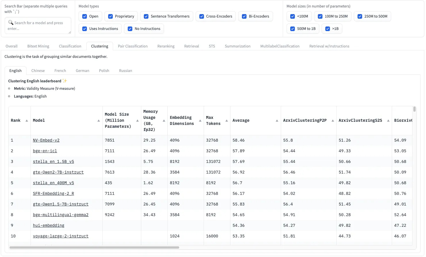
The top performers in the clustering task show an interesting trade-off. Looking at the Average column for clustering tasks, we can make informed decisions balancing performance (scores ranging from 53–58) with practical constraints like model size and memory usage. For example, while NV-Embed-v2 achieves the highest score (58.46), the stella-en-400M-v5 model offers competitive performance (56.7) with significantly lower resource requirements (435M parameters vs 7.8B).

When choosing a model, we need to balance three key factors:

1. The clustering performance (Average V-measure score)

2. Model size (which affects memory usage and inference speed)

3. Embedding dimensions (which impacts storage requirements and downstream processing)

For most practical applications, a model like stella-en-400M-v5 offers an excellent compromise — it provides strong clustering performance (55.16 average score) while being much more efficient with just 1.62GB memory usage and 8192 embedding dimensions. This makes it a practical choice unless you absolutely need the marginal performance improvement from larger models. So we will be using stella-en-400M-v5 for this exercise.

Loading the Model

from sentence_transformers import SentenceTransformer

embedding_model = SentenceTransformer('dunzhang/stella_en_400M_v5', trust_remote_code=True)
embeddings = embedding_model.encode(abstracts, show_progress_bar=True)

Creating Embeddings

embeddings = embedding_model.encode(abstracts, show_progress_bar=True)

Checking the dimensions of the resulting embedding

embeddings.shape

Output: (44949, 1024)

The following figure will help us to understand better what happened in this stage.

Document Embedding Process — Each document from our collection of 44,949 arXiv abstracts is transformed by the embedding model (stella-en-400M-v5) into a vector of 1024 dimensions.

While the MTEB leaderboard shows stella-en-400M-v5 with 8192 dimensions, the actual implementation outputs 1024-dimensional embeddings. This isn’t a discrepancy to worry about — the model developers have found that 1024 dimensions provide nearly identical performance to 8192 dimensions, with only a minuscule 0.001 difference in MTEB scores.

Stage 2: Dimensionality Reduction

High-dimensional embeddings can be computationally expensive and often contain noise. We use Uniform Manifold Approximation and Projection (UMAP) to reduce the dimensionality.

UMAP is preferred over PCA for text clustering because it:

1. Better preserves global and local structure of high-dimensional data by focusing on topological relationships rather than just linear relationships

2. Handles non-linear relationships more effectively, which is crucial for text data where semantic relationships are often non-linear

3. Generally provides better cluster separation and visualization compared to PCA

4. Scales well with large datasets while maintaining data relationships

While PCA is simpler and faster, UMAP’s ability to capture complex non-linear relationships makes it more suitable for text embedding dimensionality reduction. Let’s see the code in action.

from umap import UMAP

# We reduce the input embeddings from 1024 dimenions to 10 dimenions
umap_model = UMAP(
    n_components=10, # Reduces dimensionality while preserving essential structure
    min_dist=0.0, # Controls how tightly points cluster together
    metric='cosine', # Measures similarity between embeddings using cosine distance 
    random_state=42
)

# These parameters were chosen to optimize cluster separation while maintaining semantic relationships.
reduced_embeddings = umap_model.fit_transform(embeddings)

Checking the dimensions of the reduced embedding

reduced_embeddings.shape

Output: (44949, 10)

Pictorial representation of what exactly happened.

UMAP reduces our high-dimensional embeddings to a more manageable size

Each row still represents one document, but now with only 10 dimensions instead of 1024.

Stage 3: Clustering

Finally, we cluster the reduced embeddings using Hierarchical Density-Based Spatial Clustering of Applications with Noise (HDBSCAN).

Advantages of HDBSCAN:

• Automatically determines the number of clusters.

• Identifies outliers.

• Handles varying cluster densities.

HDBSCAN is particularly well-suited for text clustering because of its ability to work with noisy data. Let's see it in action.

from hdbscan import HDBSCAN

# We fit the model and extract the clusters
hdbscan_model = HDBSCAN(
    min_cluster_size=50, # Ensures statistically significant groupings
    metric='euclidean', # Measures distance in reduced space
    cluster_selection_method='eom' # Optimizes cluster boundary detection
).fit(reduced_embeddings)
clusters = hdbscan_model.labels_

# How many clusters did we generate?
len(set(clusters))

Number of clusters: 159

The following figure shows how documents are clustered.

HDBSCAN clusters the vectors into groups based on similarity, with documents that don’t fit well into any cluster marked as outliers.

---

Inspecting the Clusters

After applying HDBSCAN, we will proceed with inspecting the clusters by manual inspection of document samples followed by interactive 3D UMAP visualization using plotly library to understand the semantic structure of our clusters.

Manual Cluster Inspection through Document Sampling

This approach allows us to examine cluster content by printing truncated abstracts from representative documents, helping verify the semantic coherence of our clustering results.

We’ll examine the semantic coherence of our clusters by looking at representative documents from each group. Let’s go with cluster 2:

import numpy as np


# Print first three documents in cluster 0
cluster = 2 
for index in np.where(clusters==cluster)[0][:3]:
    print(abstracts[index][:300] + "... \n")

Output:

 This article presents SLAM, an Automatic Solver for Lexical Metaphors like
?d\'eshabiller* une pomme? (to undress* an apple). SLAM calculates a
conventional solution for these productions. To carry on it, SLAM has to
intersect the paradigmatic axis of the metaphorical verb ?d\'eshabiller*?,
where ... 

  Using a corpus of 17,000+ financial news reports (involving over 10M words),
we perform an analysis of the argument-distributions of the UP and DOWN verbs
used to describe movements of indices, stocks and shares. In Study 1
participants identified antonyms of these verbs in a free-response task an... 

  Contemporary research on computational processing of linguistic metaphors is
divided into two main branches: metaphor recognition and metaphor
interpretation. We take a different line of research and present an automated
method for generating conceptual metaphors from linguistic data. Given the
ge... 

Explanation:

The three abstracts shown discuss:

1. SLAM: An automatic solver for lexical metaphors

2. Analysis of UP/DOWN verb metaphors in financial news

3. Computational processing of linguistic metaphors

Based on this analysis, Cluster 2 appears to contain research papers focused on metaphors in computational linguistics.

3D UMAP Visualization: Understanding Document Cluster Distribution

This interactive visualization shows how our documents are distributed in 3D space after dimensionality reduction, with distinct clusters represented by different colors established by the clusters variable.

import pandas as pd
import plotly.express as px
from umap import UMAP

# Reduce 384-dimensional embeddings to 3 dimensions
reduced_embeddings_3d = UMAP(
   n_components=3,
   min_dist=0.0,
   metric='cosine',
   random_state=42
).fit_transform(embeddings)

# Create dataframe with 3D coordinates
df_3d = pd.DataFrame(
   reduced_embeddings_3d,
   columns=["x", "y", "z"]
)
df_3d["title"] = titles
df_3d["cluster"] = [str(c) for c in clusters]

# Create 3D scatter plot 
fig = px.scatter_3d(
   df_3d,
   x='x',
   y='y',
   z='z',
   color='cluster',
   title='3D UMAP Visualization of Document Clusters',
   opacity=0.7,
   color_continuous_scale='viridis',
   size_max=0.5,
   hover_data=['title']  # Show title on hover
)

# Update layout
fig.update_layout(
   width=900,
   height=700,
   showlegend=True
)

fig.show()

Output:

3D UMAP Visualization of arXiv NLP papers clusters based on cluster variable

Let’s zoom in to Cluster 2 to see the research paper titles of the metaphor-based NLP papers.

Zoomed-in view of Cluster 2 in 3D Space

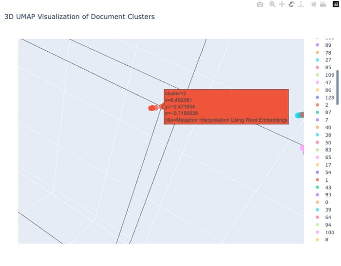
Explanation:

This visualization shows documents in cluster 2 (highlighted in red), which appear to be papers focused on metaphor interpretation using word embeddings. The 3D UMAP plot shows these documents clustered together in space, with coordinates (x=6.49, y=-2.47, z=-0.72)

• Spatial Coherence: Metaphor-related papers form a tight cluster at coordinates (x=6.49, y=-2.47, z=-0.72), indicating their semantic similarity.

• Clear Boundaries: The blue and other colored clusters visible in the background represent different research topics within the arXiv NLP dataset.

This suggests HDBSCAN successfully grouped semantically related papers focusing on metaphor analysis and processing together.

---

Conclusion

Our text clustering pipeline successfully organized 44,949 arXiv NLP papers into semantically coherent groups, as validated through both manual inspection and 3D visualization.

• Embedding Documents: Used stella-en-400M-v5 embedding model for semantic representation, which was carefully selected based on its performance metrics from the MTEB leaderboard, balanced model size (400M parameters), and optimal embedding dimensions.

• Dimensionality: Simplifying embeddings with UMAP for better clustering.

• Clustering: Grouping documents with HDBSCAN, an advanced density-based algorithm.

These three stages allowed us to effectively group related papers, exemplified by the clear metaphor research cluster in the Inspection section.

However, manual inspection of clusters becomes impractical at scale. Part 2 will introduce Topic Modeling using BERTopic library to automatically generate descriptive labels for each cluster, enabling efficient exploration of the entire document collection’s thematic structure.

---

Next Steps: Experimentation and Exploration

To deepen your understanding of text clustering, try the following:

• Experiment with Different Embedding Models: Test models from the MTEB leaderboard for accuracy and speed.

• Compare Dimensionality Reduction Techniques: Evaluate UMAP against PCA or t-SNE.

• Explore Other Clustering Algorithms: Contrast HDBSCAN with K-means or DBSCAN.

• Research Topic Modeling: Investigate BERT Topic and other topic extraction methods.

---

References

• Tutorial on Text Clustering using Sentence Transformers

• Hands-On Large Language Models — By Jay Alammar, Maarten Grootendorst

• DBSCAN vs. K-Means: Visualizing the Difference

• DBSCAN Clustering Animation