From Text to Insights: Hands-on Text Clustering and Topic Modeling — Part 2

How Can Topic Modeling Simplify Clusters into Meaningful Insights?

and

Dec 24, 2024

In the previous part of this series, we explored a hands-on approach to text clustering using a pipeline comprising embeddings, dimensionality reduction, and clustering. We demonstrated how to process 44,949 abstracts from the arXiv NLP dataset, culminating in 159 meaningful clusters. However, clustering alone only reveals groups of related documents — it doesn’t label these groups. In this article, we’ll tackle topic modeling, the process of assigning interpretable labels to clusters by extracting representative keywords.

We’ll dive into both traditional and modern approaches, implement them in Python using the BERTopic framework, and visualize results to uncover insights. Let’s get started.

What Is Topic Modeling?

Topic modeling is the art of summarizing a collection of documents by assigning descriptive keywords to represent the content. For example:

A cluster on pet-related topics might yield keywords like dog, cat, pet, and shelter.
A cooking-related cluster might include keywords like pasta, recipe, pizza, and cooking.

Traditional way to represent clustered topics as number of keywords

Unlike traditional approaches that assign a single label to each cluster, modern frameworks like BERTopic identify a collection of keywords that best describe each cluster.

Modern Framework: BERTopic

BERTopic is a modular framework for topic modeling, built to integrate seamlessly with embeddings model, dimensionality reduction, and clustering algorithms. The first part of BERTopic’s pipeline is as follows:

Embedding the Documents: Convert the documents into high-dimensional vectors. We have successfully converted each of the documents to have dimensions of 1024 using the model — stella-en-400M-v5 selected from MTEB where top clustering models are ranged by V-measure metric on Hugging Face.
Dimensionality Reduction: Reduced the embeddings from higher dimension to lower dimension— from 1024 to 10 using UMAP.
Clustering the Reduced Embeddings: We have successfully grouped the clusters using HDBSCAN which allowed us to cluster the outliers.

For detailed technical information, please refer to Part 1. To ensure clarity, all the relevant code cells will be reiterated in this article.

In the second part, keywords are extracted for each cluster to assign meaningful labels based on the extracted terms.

Overall pipeline for Topic Representation

One key benefit of this pipeline is the relative independence between the clustering process and topic representation. For example, c-TF-IDF does not rely on the specific models employed for clustering documents. So instead of UMAP, we can use PCA, DBSCAN instead of HDBSCAN, and other representation model for topic representation instead of the combination of CountVectorizer and c-TF-IDF. This design ensures a high degree of modularity across all pipeline components.

Pipeline Implementation of BERTopic

Below is the complete pipeline, from clustering to topic modeling, using the BERTopic framework.

Step 1: Install Dependencies

pip install sentence-transformers xformers bertopic datasets openai datamapplot plotly

Step 2: Load Dataset

# Load data from huggingface
from datasets import load_dataset
dataset = load_dataset("maartengr/arxiv_nlp")["train"]

# Extract metadata
abstracts = dataset["Abstracts"]
titles = dataset["Titles"]

Step 3: Generate Embeddings

Use stella_en_400M_v5 from sentence-transformers library.

from sentence_transformers import SentenceTransformer

# Create an embedding for each abstract
embedding_model = SentenceTransformer('dunzhang/stella_en_400M_v5', trust_remote_code=True)
embeddings = embedding_model.encode(abstracts, show_progress_bar=True)

Step 4: Dimensionality Reduction

Reduce high-dimensional embeddings to 10D using UMAP.

from umap import UMAP

# We reduce the input embeddings from 1024 dimenions to 10 dimenions
umap_model = UMAP(
    n_components=10, min_dist=0.0, metric='cosine', random_state=42
)
reduced_embeddings = umap_model.fit_transform(embeddings)

Step 5: Clustering

Form clusters reduced embeddings with HDBSCAN.

from hdbscan import HDBSCAN

# We fit the model and extract the clusters
hdbscan_model = HDBSCAN(
    min_cluster_size=50, metric='euclidean', cluster_selection_method='eom'
).fit(reduced_embeddings)
clusters = hdbscan_model.labels_

Step 6: Topic Modeling with BERTopic

Combine embedding, dimensionality reduction, and clustering in BERTopic.

from bertopic import BERTopic

# Train our model with our previously defined models
topic_model = BERTopic(
    embedding_model=embedding_model,
    umap_model=umap_model,
    hdbscan_model=hdbscan_model,
    verbose=True
).fit(abstracts, embeddings)

Inspect Clustered Topics

Inspect the Topics Quickly

Let’s delve into the topics generated by BERTopic:

# Fetch the topics
topic_model.get_topic_info()

Output:

Topics Generated by BERTopic: Topic IDs, Document Counts, Keywords, and Representative Documents”

Explanation:

The output from running topic_model.get_topic_info() displays detailed metadata about the topics generated by the BERTopic model. Here's an explanation of each column and the insights it provides:

Columns Explained:

1. Topic:

This column lists the unique topic IDs assigned to each cluster.
-1: Represents outliers or documents that couldn't be assigned to any specific cluster.
Other values (0, 1, 2, ...) correspond to the generated topics.

2. Count:

Indicates the number of documents assigned to each topic.
Larger counts suggest dominant or more popular topics, while smaller counts could indicate niche or less discussed topics.
For example, Topic -1 has 13,040 documents, indicating a large set of outliers, while Topic 0 has 2,482 documents, making it a major identified cluster.

3. Name:

Provides a unique identifier or label for the topic, typically structured as <topic_id>_<keywords>.
The keywords included in the name give a quick overview of the main terms associated with that topic.
Example: Topic 1_medical_clinical_biomedical_patient reflects its focus on medical and clinical-related content.

4. Representation:

This column lists the extracted keywords for each topic. These keywords are derived using the c-TF-IDF method or other topic representation methods and summarize the core content of the topic.
For example:
- Topic 0: Keywords such as speech, asr, recognition, end, acoustic indicate its focus on speech recognition systems.
- Topic 155: Keywords like emoji, emojis, emoticons, sentiment suggest the topic pertains to emoji usage and sentiment analysis.

5. Representative_Docs:

Displays a sample of representative documents (or document abstracts) from each topic.
These documents serve as examples of what type of content belongs to the cluster, helping users understand the context and meaning of the topic.
Example: For Topic 1_medical_clinical_biomedical_patient, a representative document might discuss distributed representations of medical concepts.

Insights from the Results

1. Dominant Topics:

Topic 0 is the largest cluster with 2,482 documents, focusing on speech recognition (speech, asr, recognition, acoustic). This likely represents a significant research area within the dataset.

2. Niche Topics:

Topics like 157_deception_reviews_deceptive_fake (51 documents) or 153_translation_english_en_submission (53 documents) indicate smaller clusters dealing with specific subjects such as deceptive reviews and translation systems.

3. Outliers:

Topic -1 is labeled as an outlier cluster with generic keywords (of, the, and, to) and includes 13,040 documents. This topic may include:
- Documents with no clear thematic similarity.
- Noise or irrelevant data.

4. Keyword Distribution:

Keywords provide a concise summary of the topics’ themes. For example:
- Summarization, summaries, summary, abstractive for Topic 3 indicates a focus on text summarization techniques.
- Medical, clinical, biomedical for Topic 1 clearly points to healthcare-related research.

5. Understanding Representative Documents:

The Representative_Docs column offers a direct way to understand the real-world content behind each cluster. These documents are crucial for verifying the accuracy and coherence of the generated topics.

Inspect Topics Individually

We can also inspect topics individually using get_topic(<topic_number>) . Example as follows:

topic_model.get_topic(15)

Output:

[('morphological', 0.03180901561754959),
 ('subword', 0.021767213735360412),
 ('character', 0.01806202274504348),
 ('tokenization', 0.013643008991703304),
 ('languages', 0.011831199917118796),
 ('bpe', 0.011474163603948092),
 ('word', 0.011269847039854718),
 ('segmentation', 0.011219194104966166),
 ('morphology', 0.011096301412965344),
 ('morphologically', 0.01090045014679196)]

Explanation:

Topic 15 includes the keywords “subword,” “tokenization,” and “bpe” (Byte Pair Encoding). These keywords suggest that the topic primarily focuses on tokenization.

We can use find_topics(<topic_name_we_are_interested>) to search for specific topics related to a given search term. Let’s try it out:

topic_model.find_topics("Large Language Models")

Output:

([11, -1, 104, 50, 52],
 [0.7391623, 0.7299156, 0.72964495, 0.71527004, 0.69776237])

Explanation:

A higher score (closer to 1) means the topic is more relevant to the search term.
Topic 11 has the highest relevance score (0.73), while Topic 52 has the lowest in this result set (0.69).

Let’s inspect further to confirm if the topic is about Large Language Models.

topic_model.get_topic(11)

Output:

[('evaluation', 0.017788030494504652),
 ('metrics', 0.013616483806350986),
 ('llms', 0.012587065788634971),
 ('human', 0.010760840609925439),
 ('chatgpt', 0.01052913018463233),
 ('nlg', 0.009619504603365265),
 ('llm', 0.007265654969843764),
 ('language', 0.007094052507181346),
 ('generation', 0.006545947578436024),
 ('of', 0.0063761418431831154)]

Explanation:

We can see the keywords — “llms”, “generation”, “language”, “chatgpt”. This confirms that the topic is about Large Language Models.

We further can confirm using topic_model.topics_[titles.index(<title_of_the_abstract>)]

topic_model.topics_[titles.index("A Survey on Evaluation of Large Language Models")]

Output is 11.

Visual Inspection

Visualize the Topics in 3D Space

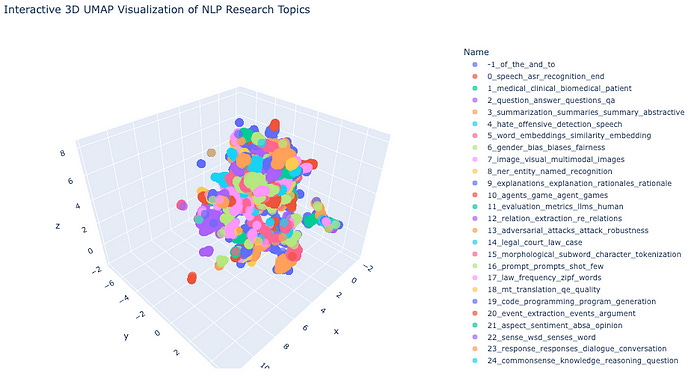
BERTopic provides inbuilt topic_model.visualize_documents to visualize. There is a limitation to it though — just views 2D. Therefore, we will use raw code and use plotly library to view 3D (it is much cooler 😛). We will also explore 2D plot as well after this section.

# Import necessary libraries
import pandas as pd
import plotly.express as px
from umap import UMAP

# Step 1: Dimensionality Reduction
# Reduce high-dimensional embeddings (1024D) to 3D space for visualization
# UMAP is chosen for its ability to preserve both local and global structure
reduced_embeddings_3d = UMAP(
    n_components=3,    # Target 3 dimensions for 3D visualization
    min_dist=0.0,      # Minimum distance between points, 0.0 for tighter clusters
    metric='cosine',   # Cosine similarity is well-suited for text embeddings
    random_state=42    # Set seed for reproducibility
).fit_transform(embeddings)

# Step 2: Create DataFrame with 3D Coordinates
# Transform UMAP output into a pandas DataFrame for easier manipulation
df_3d = pd.DataFrame(
    reduced_embeddings_3d,
    columns=["x", "y", "z"]  # Name dimensions for clarity
)
df_3d["title"] = titles                         # Add document titles
df_3d["cluster"] = [str(c) for c in clusters]   # Add cluster labels

# Step 3: Prepare DataFrames for Merging
# Convert data types to ensure consistent joining
topic_df = topic_model.get_topic_info()         # Get topic modeling results
topic_df['Topic'] = topic_df['Topic'].astype(int)
df_3d['cluster'] = df_3d['cluster'].astype(int)

# Step 4: Merge Topic Information with Coordinates
# Combine topic information with 3D coordinates using inner join
merged_df = topic_df.merge(
    df_3d,
    left_on='Topic',
    right_on='cluster',
    how='inner'
)

# Step 5: Select Relevant Columns
# Keep only necessary columns for visualization
columns_to_keep = ['Name', 'x', 'y', 'z', 'title']
final_df = merged_df[columns_to_keep]

# Step 6: Create Interactive 3D Visualization
# Use Plotly Express for an interactive 3D scatter plot
fig = px.scatter_3d(
    final_df,
    x='x',
    y='y',
    z='z',
    color='Name',      # Color points by topic name
    title='Interactive 3D UMAP Visualization of NLP Research Topics',
    opacity=0.7,       # Set partial transparency for better visibility
    color_continuous_scale='viridis',  # Use viridis color palette
    size_max=0.5,      # Control point size
    hover_data=['title']  # Show document title on hover
)

# Step 7: Customize Plot Layout
# Adjust plot dimensions and enable legend
fig.update_layout(
    width=1200,
    height=700,
    showlegend=True
)

# Display the interactive plot
fig.show()

Output:

3D UMAP Visualization of arXiv NLP Papers: Topics automatically labeled by BERTopic using representative keywords.

Let’s hover over each cluster to explore the titles of the abstract based on our topic interest.

Hovered over the cluster — `0_speech_asr_recognition_end over 3D space`

Explanation:

Rather than determining manually, we can see the topic names assigned by BERTopic for each of the clusters visually in 3D Space.

There are various other ways too for visualization facilitated by BERTopic. Let’s explore.

Visualize the Topics in 2D

topic_model.visualize_topics()

Output:

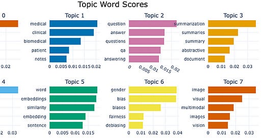
2D Space representing how far are each of the clusters

topic_model.visualize_barchart()

Output:

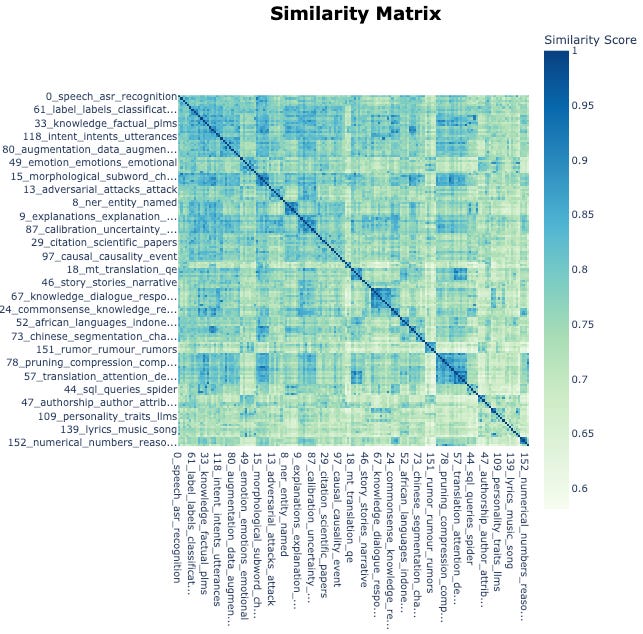
# Visualize relationships between topics
topic_model.visualize_heatmap(n_clusters=30)

Output:

Visualizing all of the topics that are similar to each other

Conclusion

In this article, we:

Transformed clusters of arXiv NLP paper abstracts into actionable insights using BERTopic for topic modeling.
Descriptive keywords as cluster title: Assigned descriptive keywords to each cluster, enabling effective understanding of vast datasets.
Manual inspection no more required: Eliminated the need for manual inspection by automating the topic assignment process.

Limitations of the current method:

Relies on the Bag-of-Words model and counting schemes like TF-IDF.
Fails to capture semantic and contextual nuances inherent in language.
Treats words as independent tokens without considering their meanings or relationships.
Results in topics that may lack depth and fail to represent the true essence of the underlying data.

Next Steps: Embracing Semantic Representations

To deepen your understanding of topic modeling using BERTopic, try to use different topic representation models. Take full advantage of modular nature of this modern library and try out methods — Jeiba or POS instead of CountVectorizer and the combination of BM25 + class-based TF-IDF that we have used. This will allow us to get the best results if we use it for production. Also, try other visualization methods provided by BERTopic for further inspection.

In the next part of this series, we will:

Address the limitations by integrating advanced representation models into our topic modeling pipeline.
Explore how incorporating semantic contextual meaning can refine topic representations.
Delve into leveraging generative models — Large Language Models (LLMs) — to enhance our insights.

References

Thank you for reading! If you found this tutorial helpful, please share it with others and leave a comment below.

Vizuara’s Substack

Discussion about this post