From Words to Vectors: Understanding Word Embeddings in NLP

From static vectors to contextual understanding — exploring Word2Vec, embeddings, and Transformer models

Introduction

How can a computer begin to grasp the meaning of a simple word or sentence? This challenge lies at the heart of natural language processing, where computers require numbers – not letters or words – to represent language. A crucial solution is to encode each word as a numerical vector that captures its meaning and context. In other words, word embeddings provide a powerful way to map words into a multi-dimensional space where linguistic relationships are preserved. This blog will explore how word embeddings bridge human language and machine computation, using clear visualizations and a step-by-step approach to make these foundational concepts accessible and academically rigorous.

Why Turn Words into Numbers?

Think about how a computer “reads” text. Computers ultimately work with numbers, not letters or words. When we type words like "dog" or "love" into a computer, it doesn’t understand them the way we do. Computers operate at a fundamental level using numbers — binary digits (0s and 1s) — not letters or human language. So even though we’re feeding it natural language, the machine needs a way to interpret that input numerically.

So if we want a machine to understand language, we need to convert words into numbers.

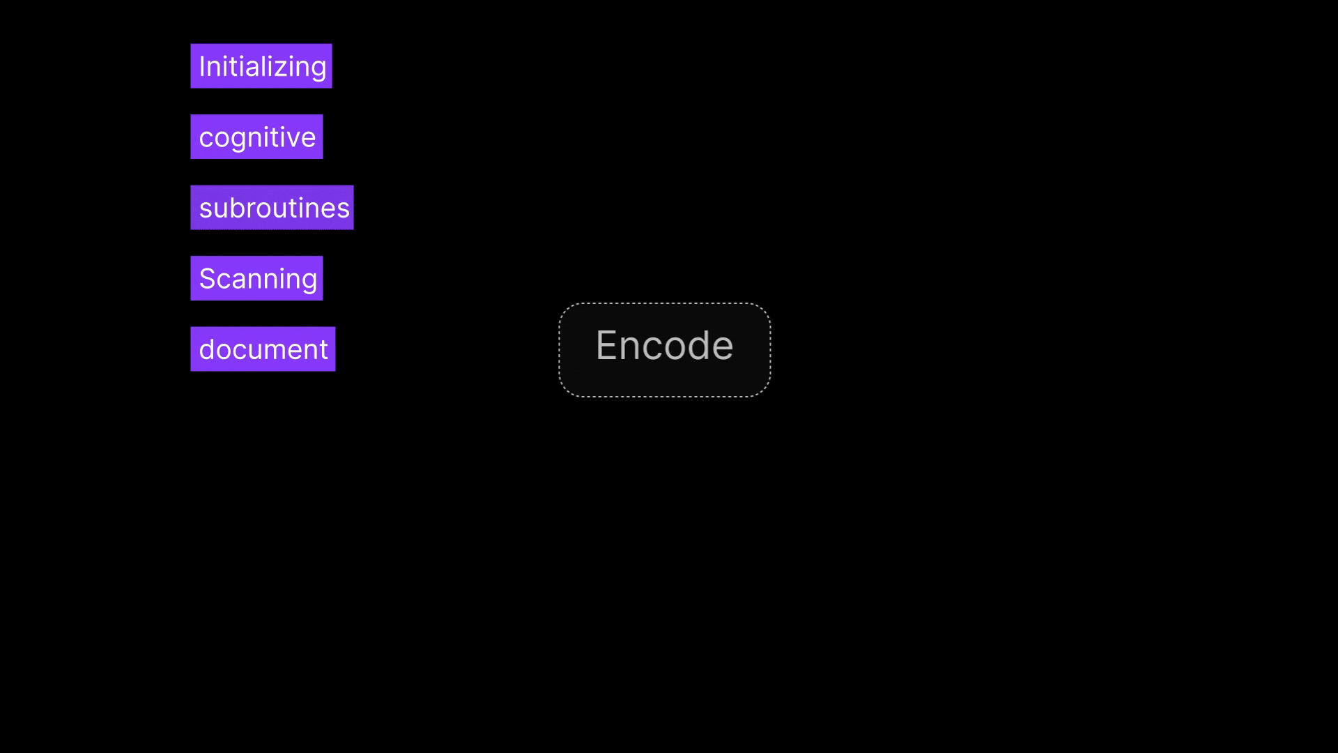
To bridge this gap, we must convert human language into a form that a machine can work with — numerical values. This process is known as encoding. Encoding takes text (words, characters, sentences) and maps it into numeric representations, such as binary or vectors, that the computer can manipulate mathematically.

Early on, a simple solution was to assign each word an ID number (like an index in a dictionary).

A straightforward approach in the early days of NLP was to treat each word as a distinct symbol and assign it a unique numeric ID. This is much like how a dictionary works — each word gets its own slot or position. For example:

For example, we might say

• “apple” is 1

• “banana” is 2

• “cat” is 3

and so on. This gives each word a unique numeric identifier.

This technique is called integer encoding or token indexing. While simple and useful for building basic vocabularies, this method has a major shortcoming: the numbers carry no semantic value. There’s no inherent meaning in the fact that “cat” is 3 or “apple” is 1.

The numeric IDs are just labels. The model has no clue that "cat" and "dog" are both animals or that they’re more related to each other than to "banana". The system lacks any understanding of context or relationships. It treats each word as entirely distinct and unrelated — which is not how language works.

The number 3 doesn’t tell the computer that “cat” is an animal or that it’s more similar to a “dog” than to a “banana.” It’s just a label.

“Cat” vector should be closer to “Dog”

One Hot Encoding

Imagine telling a machine that "cat" is represented by 3. This number tells it nothing about the word itself. The computer doesn’t understand that “cat” might be more like “dog” than “banana”. It's like assigning jersey numbers to players – useful for identity, but meaningless in terms of skill, position, or teamwork.

To overcome this, researchers introduced one-hot encoding, a method that doesn’t rank words with numeric values, but instead gives each word its own exclusive position in a large binary vector.

To preserve more information, researchers tried representing words as one-hot vectors.

In a one-hot vector, each word is represented by a vector filled with 0s, except for a single 1 in the position assigned to that word. For example:

• "apple" → [1, 0, 0, 0, 0]

• "banana" → [0, 1, 0, 0, 0]

• "cat" → [0, 0, 1, 0, 0]

This eliminates the unintended assumption of ranking or value between words. Every word is now treated as equally different — they’re all orthogonal (perpendicular) in vector space.

A one-hot vector is like a long binary code for each word: mostly zeros, with a single 1 at the position corresponding to that word.

If “cat” is the 3rd word in our vocabulary, its one-hot vector might look like [0, 0, 1, 0, 0, ...] (with a 1 in the 3rd slot).

Now imagine applying one-hot encoding to an entire sentence. If “cat” is the third word in our vocabulary, its one-hot representation might be [0, 0, 1, 0, 0]. This is fine for small vocabularies. But real-world applications often deal with tens or hundreds of thousands of words. That means each vector could be extremely long, with only one non-zero element. It get very large and sparse (a long list of zeros) if you have a lot of words .

Sparse Vector

This becomes inefficient both in memory and computation. These vectors are called sparse — full of zeros. And like token IDs, one-hot vectors don’t carry any information about word meaning or relationships.

More importantly, they don’t capture any relationships or meanings – a one-hot encoding “thinks” that cat is as unrelated to dog as it is to table, since every word’s vector is equally different (sharing no common 1s) . In other words, one-hot vectors do not capture meaning.

Bag of Words

Another early approach was the Bag-of-Words (BoW) model.

Instead of representing individual words, BoW represents an entire piece of text (like a sentence or document) by counting the occurrences of each word. You basically make a big vocabulary list and count how many times each word appears, turning the text into a numerical frequency vector. This captures which words are present and how often, but it ignores the order of words completely .

If you have the sentences "dog bites man" and "man bites dog," a basic bag-of-words representation would treat them as the same thing, since both contain one "dog", one "man", and one "bites."

Clearly, word order matters for meaning (who bit whom in this case!), and BoW loses that information. Moreover, like one-hot vectors, BoW vectors can be very high-dimensional and mostly zeros (especially for long vocabulary lists).

The shortcomings of these early methods made it clear that we needed a better way to turn text into numbers – a way that captures meaning, context, and relationships between words, not just identity.

Meaning Through Context: The Distributional Hypothesis

How can we give the computer a sense of what words mean? One powerful idea from linguistics is that meaning comes from context.

“You shall know a word by the company it keeps.” - J.R. Firth

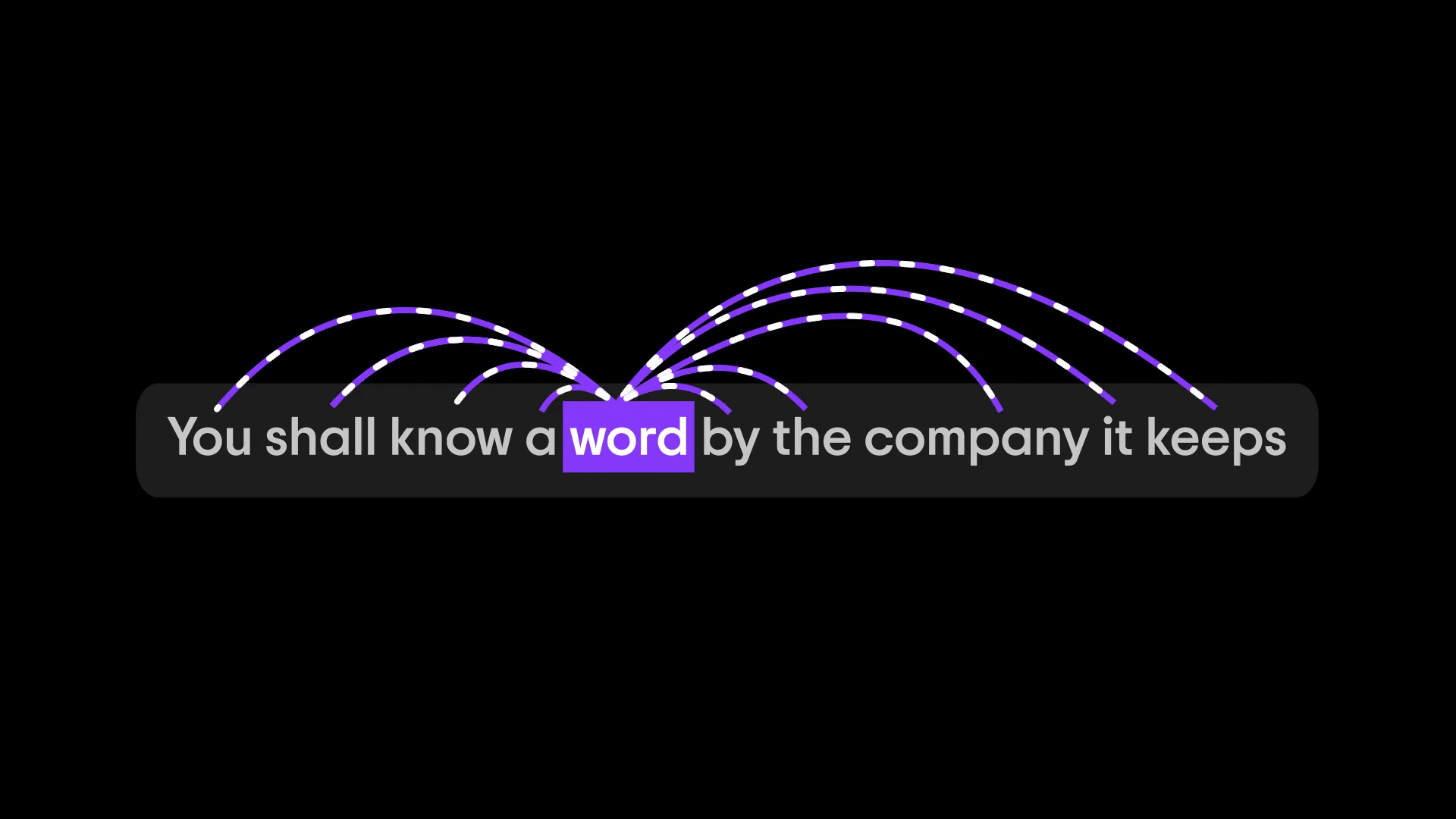
There’s a famous saying by linguist J.R. Firth: “You shall know a word by the company it keeps.” In simple terms, this means you can often infer the meaning of a word by looking at the words around it.

Distributional hypothesis : words appearing in similar contexts tend to have similar meanings.

This is known as the distributional hypothesis, which states that words appearing in similar contexts tend to have similar meanings.

Think about how you deduce the meaning of an unfamiliar word when reading.

If you see a sentence, "The glorp is barking and wagging its tail," you can guess that “glorp” might be some kind of animal, probably a dog, even if you’ve never heard that word before.

Computer thinking: 'It must be some animal, like a dog

The Word ‘dog’ appears near. ‘barking’, ‘wagging’, and ‘tail’, showing how surrounding words provide strong contextual clues about its meaning

Why? Because the context (“barking”, “wagging its tail”) gives it away.

Similarly, if two different words often appear in the same sort of contexts, there’s a good chance they relate to similar things.

'Doctor', 'patient', and 'hospital' cluster together, while 'guitar' stands apart—showing meaning through context.

For instance, the words "doctor" and "nurse" both appear frequently near words like "hospital" or "patient", so a computer could learn that they are related in meaning. On the other hand, "doctor" and "guitar" rarely share contexts, so their meanings are likely unrelated.This insight suggests a strategy: represent each word by the contexts in which it appears. If we can encode the surrounding words into a vector, we get a numeric representation that reflects usage and thus meaning.

"Earlier methods relied on large co-occurrence tables to capture word relationships”

Early count-based approaches did this by constructing huge tables (matrices) of word co-occurrences (how often each word appears next to each other word) and then factorizing or compressing those tables to get dense vectors. But an even more effective strategy turned out to be letting a machine learning model learn word vectors from context automatically. This is where neural network-based embeddings came into play.

Learning Word Embeddings: Word2Vec

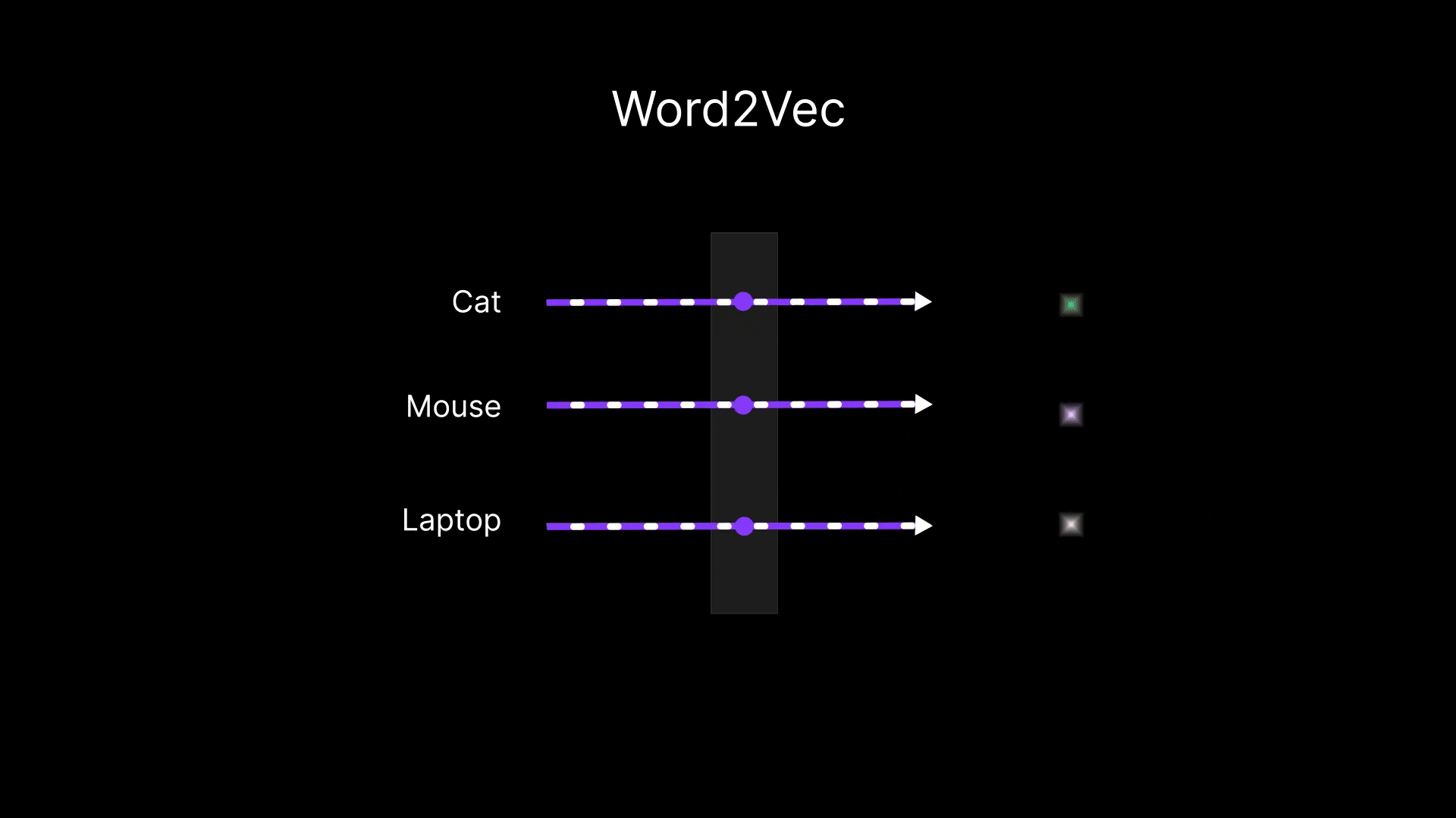
A breakthrough in making word meaning numeric came with models like Word2Vec, created by a team at Google in 2013. Word2Vec is not a single algorithm but a family of related approaches to learn word embeddings (dense vector representations) from a large corpus of text.

The core idea is straightforward and follows the context = meaning principle: use the surrounding words (context) to predict a target word, or vice versa.

In doing so, the model learns vectors for words that make those predictions accurate. Over time, those vectors come to encode semantic information, because to predict a word from its neighbors (or neighbors from the word), the model has to pick up on which words tend to go together.

Word2Vec popularized two training strategies that implement this idea: Continuous Bag of Words (CBOW) and Skip-Gram. They are like two opposite ways to solve a fill-in-the-blank puzzle:

CBOW (Continuous Bag of Words)

Imagine taking a sentence and hiding one word, then asking the model to guess the missing word based on the other words around it.

For example, in "The cat ___ on the mat", the model should predict "sat" from the context ["The", "cat", "on", "the", "mat"]. CBOW treats the surrounding context words as input and tries to predict the target word. Essentially, it learns to guess a word from its neighbors. To succeed, the model must internalize the contextual clues – this pressure causes it to learn meaningful word vectors in its hidden layer. Words that appear in similar contexts (and could plausibly fill in similar blanks) end up with similar vector representations.

SKIP GRAM

Now flip the problem around. In Skip-Gram, the model sees one word and tries to predict the words that are likely to appear around it

For example, given the word "coffee", the model might try to predict that words like "morning", "mug", or "bean" often occur nearby. In practice, the training takes each word in a sentence as the center and tries to guess its context words. Skip-gram is essentially learning to guess the neighbors from the word. This also forces the model to learn vectors that position similar words in a way that they have similar neighboring distributions.

Both CBOW and Skip-Gram are just simple neural networks with one hidden layer. There’s nothing obviously magical in their architecture – the magic comes from training on millions of sentences. Over many iterations, the model adjusts the word vectors to better predict missing words or neighbors. The end result is a set of vectors (one for each word in the vocabulary) where words that “live” in similar contexts are closer together in vector space, capturing a lot of subtle semantic and syntactic relationships.

For example, after training, the vector for “king” might end up near “queen”, “prince”, and “royal”, while “banana” would end up closer to “apple”, “fruit”, or “yellow”.

One famous demonstration of Word2Vec’s power is that these word vectors can sometimes capture analogies through arithmetic.

Let’s judge a word based on some certain parameters

King - Man + Woman ≈ Queen

we have king , man , woman and queen so we have a slider in the range of 0 to 10.

Now king is very rich that why the value of the first vector could be 9, for the gender male the value will go at 0, king is very powerful that’s why the power value could be 9.5

Let’s apply the same for man then the same for women and here and then for the word queen

To better understand these relationships, let’s plot the vectors for king, queen, man, and woman in a 2D space. This simplified visualization helps illustrate how word embeddings capture analogies as directional movements in vector space.

Before we get to "king - man + woman ≈ queen", it's helpful to understand a simpler but equally powerful form: "queen - woman = king - man". This equation shows that the relationship between "queen" and "woman" is the same as the relationship between "king" and "man". In other words, becoming a "queen" from a "woman" involves the same conceptual leap — royalty — as going from "man" to "king". These relationships are captured as directions between word vectors, allowing models to understand analogies through geometry.

One of the most fascinating things about word embeddings is how they can capture relationships between words mathematically.

A famous example is the equation "king - man + woman ≈ queen".

This means that if we take the vector for "king", subtract the concept of "man", and add "woman", we get a new vector that's very close to "queen". It’s like teaching the model that the difference between "king" and "queen" is the same as the difference between "man" and "woman".

This shows how word embeddings can understand not just meanings, but also relationships between words — almost like reasoning with language!

The model has learned aspects of the relationships like gender in its vector geometry. While this “analogy math” is a fun aside, the key takeaway is that word embeddings transform raw text into a kind of geometric space of meanings. Each word becomes a point in a multi-dimensional space, and words with similar meanings cluster together in that space. In our new numeric representation, “happy” might be right next to “joyful,” while “apple” would be far from “dog” . By turning words into these learned vectors, we’ve given computers a way to calculate word similarities and even associations.

Comparing Word Meanings with Cosine Similarity

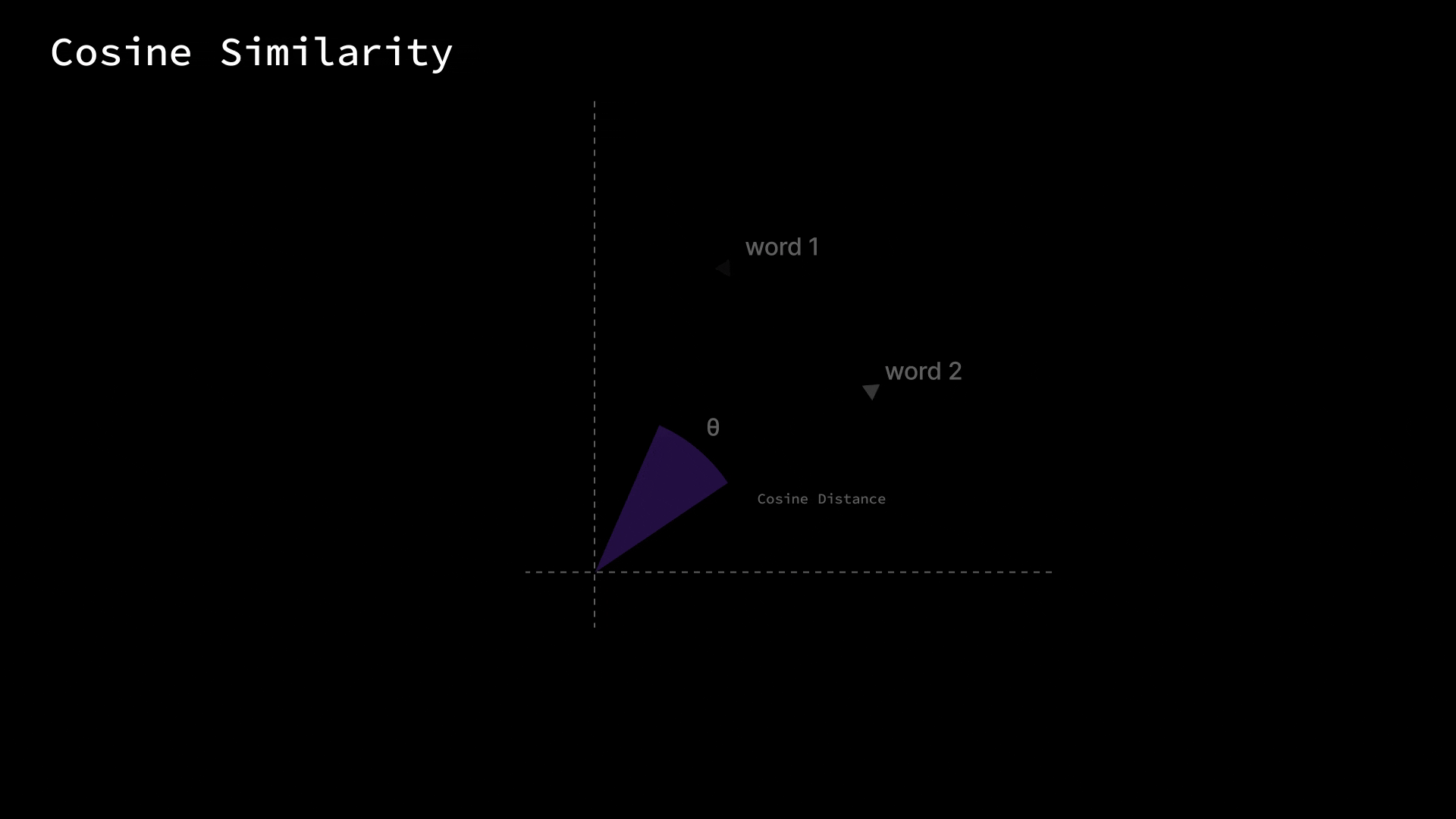
Once we have words as vectors, how do we actually measure if two words are similar in meaning? One common measure is cosine similarity.

Without diving into heavy math, cosine similarity looks at the angle between two word vectors, not their length. Imagine each word vector as an arrow pointing from the origin of this multi-dimensional space to the point for that word.

Cosine similarity asks: how close is the direction of Arrow A to Arrow B?

If two word vectors point in very similar directions (small angle between them), the cosine similarity is high (close to 1.0), meaning the words are likely related.

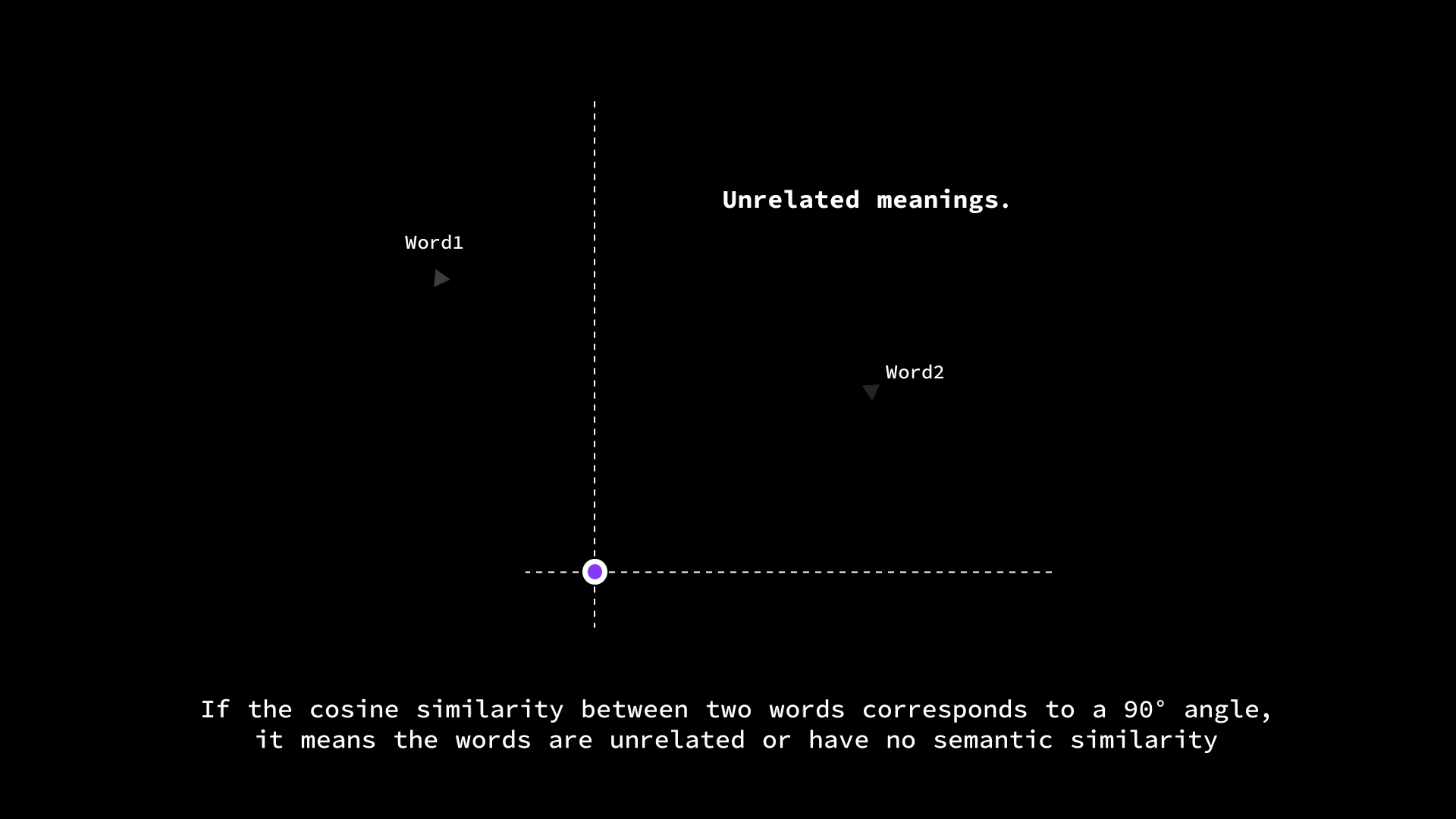
If they’re at 90° (perpendicular), the cosine is 0, indicating no particular similarity.

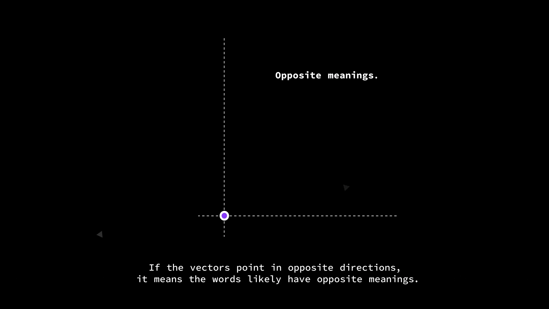
And if they point in opposite directions (180° apart), the cosine similarity is -1 (which in word terms might indicate opposites, though in practice embeddings usually aren’t so neatly antonymous).

The nice thing about cosine similarity is that it ignores the magnitude of the vectors and focuses only on orientation. Why is that useful? Because in training, some words might get larger vector values than others (say, very common words might have higher magnitudes), but what really encodes meaning is the direction (the pattern of values across dimensions). Cosine similarity effectively normalizes that out. In simpler terms, it checks how much two words “point in the same direction” in the meaning space.

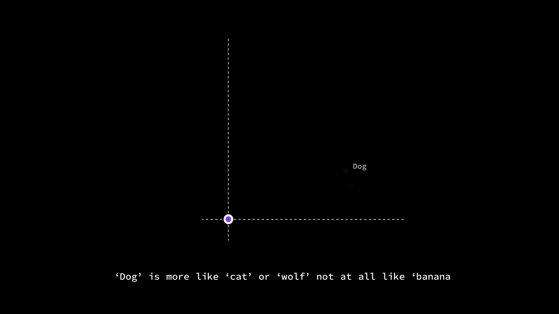
So, if we want to find which word is most similar to "dog" in our vocabulary, we can compute the cosine similarity between dog’s vector and every other word’s vector – we might find “cat” has a similarity of 0.8, “wolf” 0.75, “banana” maybe 0.2. That aligns with our intuitive understanding that dog is more like a cat or wolf, and not at all like a banana. By using measures like cosine similarity on embeddings, LLMs and other NLP systems can quantitatively compare meanings – for example, to find synonyms, to detect if a piece of text matches a query, or to cluster words by topics.

Interpretability: What Do Word Embeddings Really Mean?

By now, it’s well understood that every word in modern Natural Language Processing (NLP) models is represented as a vector of numbers — commonly referred to as a word embedding. But this raises an important question:

What do these numbers actually mean?

Why does each word have a different vector?

This is where the concept of interpretability comes into play. Interpretability in word embeddings is about uncovering the hidden structure behind these vectors, trying to understand what semantic or syntactic features each dimension might represent.

We don't know exactly what each number stands for, since these vectors are learned in an unsupervised way. However, by visualizing the vectors — such as plotting heatmaps and color-coding the values — we can begin to form hypotheses.

For example, we might use a color gradient where:

• Highly negative values appear purple

• Highly positive values appear red

Let’s say we visualize just the first 10 dimensions out of a typical 300-dimensional embedding. When we do this, an interesting pattern might emerge.

Case Study 1: Living vs. Non-Living — man, woman, boy, girl, banana, water

In this example, we explore a set of words that belong to two broad categories:

• Living entities: man, woman, boy, girl

• Non-living objects: banana, water

Observation:

In dimension 6, all the words that represent living entities (such as “man”, “woman”, “boy”, “girl”) show strong negative (purple) values, whereas non-living objects like “banana” and “water” do not show such values.

This pattern suggests that dimension 6 may be encoding some latent attribute related to the concept of "life" or "animacy". It appears to distinguish between things that are alive versus inanimate objects.

We can’t definitively say that dimension 6 represents living vs. non-living. This is simply a hypothesis formed by observing patterns in the data. The dimension could also represent other correlated attributes, such as "agency", "interaction", or "social presence" — features that are commonly associated with living things in language usage.

Case Study 2: Emotions — happy, joyful, sad

Let’s move to a group of emotional words:

• Positive: happy, joyful

• Negative: sad

These words are plotted across 10 dimensions, and their values are color-coded using a gradient that helps us visually interpret their structure.

Observation:

• Across most dimensions, happy and joyful show very similar patterns — values across dimensions like d1, d2, d3, and d7 are nearly aligned.

• However, there's an important distinction at dimension d6:

  • happy: 0.04

  • joyful: 0.17

  • sad: 0.86 — much higher than the others.

This suggests that dimension d6 might be playing a role in encoding emotional polarity, potentially distinguishing joy from sadness. However, this is only a hypothesis. It’s also possible that d6 represents something correlated but not directly interpretable, like emotional intensity or context frequency.

Case Study 3: Life Stages — baby, child, adult, teenager

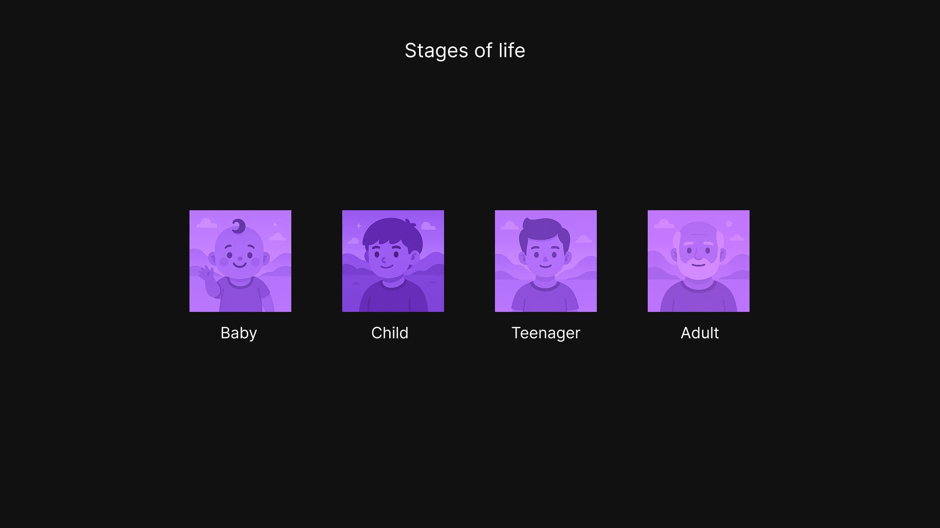
Next, let’s analyze a completely different semantic group: human life stages.

Observation:

• All four words (baby, child, adult, teenager) have notably similar vectors, especially around dimensions d2, d3, and d5.

• One interesting pattern appears at dimension d8:

  • baby: 1.30

  • child: 1.17

  • adult: 0.79

  • teenager: 0.98

This descending trend could hypothetically relate to something like "available free time" — a concept that intuitively decreases as one transitions from infancy to adulthood. Again, this is purely speculative. These values might correspond to a range of abstract linguistic or cultural associations learned from the training data.

Takeaway:

Even though we cannot definitively assign meanings to individual dimensions, consistent patterns across word groups suggest that the model is capturing shared features relevant to those categories.

Final Thoughts: Can Embedding Dimensions Be Interpreted?

A common misconception is that each dimension in a word vector represents a specific interpretable trait (e.g., "gender", "age", "positivity"). In reality:

• Embeddings are learned in an unsupervised way, and the dimensions are not explicitly labeled.

• Still, similar meanings lead to similar vector compositions.

• Interpretability often comes from relative comparisons, not from absolute values.

So while it’s tempting to say “dimension 6 represents joy” or “dimension 8 represents age,” these are merely hypotheses formed from visual patterns and domain knowledge. We can never be completely certain — but we can observe and reason.

While word embeddings don’t offer explicit labels for each dimension, patterns across similar words reveal that they do capture meaningful relationships. These consistent patterns help us interpret embeddings and trust their use in real-world NLP tasks even if the exact meaning of each dimension remains uncertain.

Beyond Single-Meaning Vectors: Contextual Embeddings (Transformers)

Word2Vec and similar embedding methods (like GloVe or FastText) were game-changers. However, they have a limitation: each word gets one static vector, no matter where or how it’s used.

But many words are polysemous – they have multiple meanings. The word “bank” in “bank account” vs “river bank” is a classic example: one is about finance, the other about a river’s edge.

Look at the above image the first says, “Mayank is sitting quietly on the river bank, watching the water flow,” while the second reads, “Mayank is robbing the bank downtown with a mask on his face.” Both use the word “bank,” yet one refers to the edge of a river, and the other to a financial institution.

This simple contrast reveals a major flaw in traditional models like Word2Vec: they treat “bank” as a single vector, regardless of context. So whether it's about nature or finance, Word2Vec assigns the same embedding, which can confuse models that rely on these vectors.

In a Word2Vec embedding space, “bank” has to be a single point, so the model might place it somewhere between the two meanings, or closer to the more frequent meaning. This is not ideal for understanding sentences, because the computer can’t fully tell which sense is meant just from that one vector. In fact, with static embeddings, each word has only one vector, so it cannot explicitly distinguish different meanings in different contexts.

Modern transformer-based models like BERT (Bidirectional Encoder Representations from Transformers) and GPT (Generative Pre-trained Transformer) solve this by using contextual embeddings. Instead of a fixed vector per word type, these models generate a fresh vector for each word token based on the sentence it’s in. In other words, the representation of "bank" in a finance context will be different from the representation of "bank" in a river context.

How do they do this? They use deep neural networks (Transformers) that look at the entire sentence (and even surrounding sentences) when encoding a word. The result is that the meaning of the word as used is captured in its vector. BERT, for example, reads a sentence and produces an embedding for each word position. So the same word can have multiple possible vectors depending on its “company” in that instance – fulfilling Firth’s context idea in a very direct way.

What’s remarkable is that these contextual embeddings allow one model to handle many nuances of language.

If you ask BERT to fill in the blank for "I went to the ___ to deposit money," it knows the blank should be something like "bank" (finance sense). If you instead say "I sat on the ___ by the water," it will predict "bank" (river sense) as a likely word, and it knows these are different meanings.

Under the hood, the internal vector for "bank" in the first sentence will be closer to other finance-related words, and in the second sentence it will be closer to river-related words. We’ve moved from a single static map of words to a flexible, context-sensitive mapping.

Transformer models use these embeddings in every layer of their network and especially as part of their output or attention calculations. Essentially, contextual embeddings allow language models to disambiguate word meanings on the fly, making them much more powerful for understanding text than any static lookup table of word vectors could be.

Conclusion

Word embeddings have proven to be a pivotal bridge between human language and machine understanding. The evolution from treating words as arbitrary IDs (or one-hot tokens) to encoding their nuanced contexts in modern Transformer models represents a major leap forward in natural language processing. While the idea of placing words into a mathematical vector space can seem abstract, our step-by-step visual approach has shown that these concepts can be made concrete and intuitive. Mastering embeddings is not the end of the story but a stepping stone – these vector representations power countless NLP applications today and inspire curiosity about even deeper models and future advancements beyond the embedding space.

---

I’m also building ML, MLOps and LLM projects, sharing and discussing them on LinkedIn and Twitter. If you’re someone curious about these topics, I’d love to connect with you all!

LinkedIn : www.linkedin.com/in/mayankpratapsingh022

Twitter/X : x.com/Mayank_022

Thanks for joining the journey so far.