
Hands-on RL Bootcamp Lecture 1
A practical and easy-to-follow program from Q-learning and DQNs to RLHF and GRPO!

In this lecture, we began our journey by first understanding classical reinforcement learning.
The Reinforcement Learning Problem
To understand the RL problem, we first need to understand how different it is from supervised learning and unsupervised learning.
First, let's look at supervised learning.
The objective of supervised learning is to be able to generalize or extrapolate in situations not present in the training dataset. We'll look at the example below.
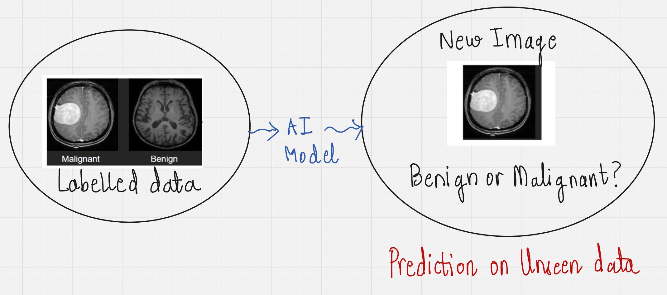
In this example, we have provided a labeled dataset containing MRI scans for “malignant” and “benign” tumors. We then train our AI model to understand patterns from these images and learn to distinguish between both types of tumors.
Now, unsupervised learning is something completely different. Here, our objective is to find structures that are hidden in collections of unlabeled data. Have a look at the example below.
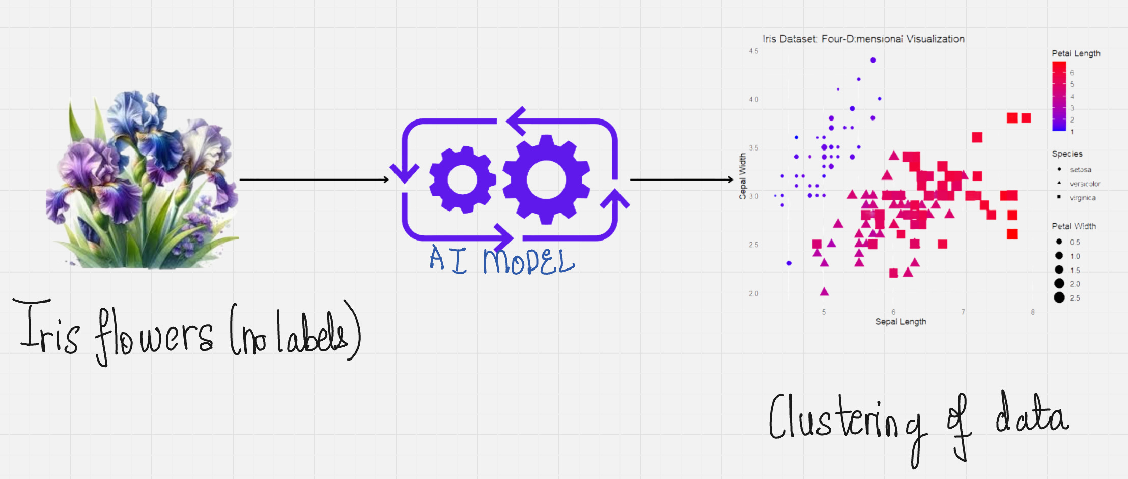
In this example, we have provided a dataset for Iris flowers without any labels. Our model learns to identify groups or clusters in the data by grouping together items having similar characteristics.
Now let us understand how reinforcement learning compares to both the categories discussed above.
First, let us start with the labeling of data.
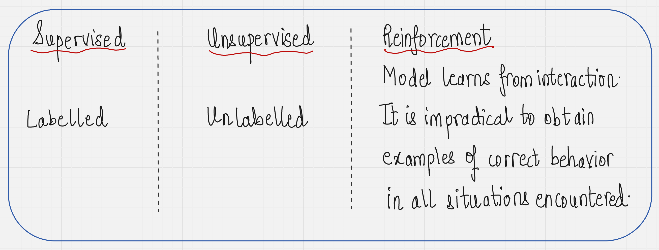
In reinforcement learning, our model learns from interactions with the environment. While interacting with the environment, it is impractical to obtain examples of correct behavior in all the situations which are encountered.
Since there is no data that is provided to the model as such.
Next, we will look at the objective of the reinforcement learning problem and how it differs from the two categories we saw before.
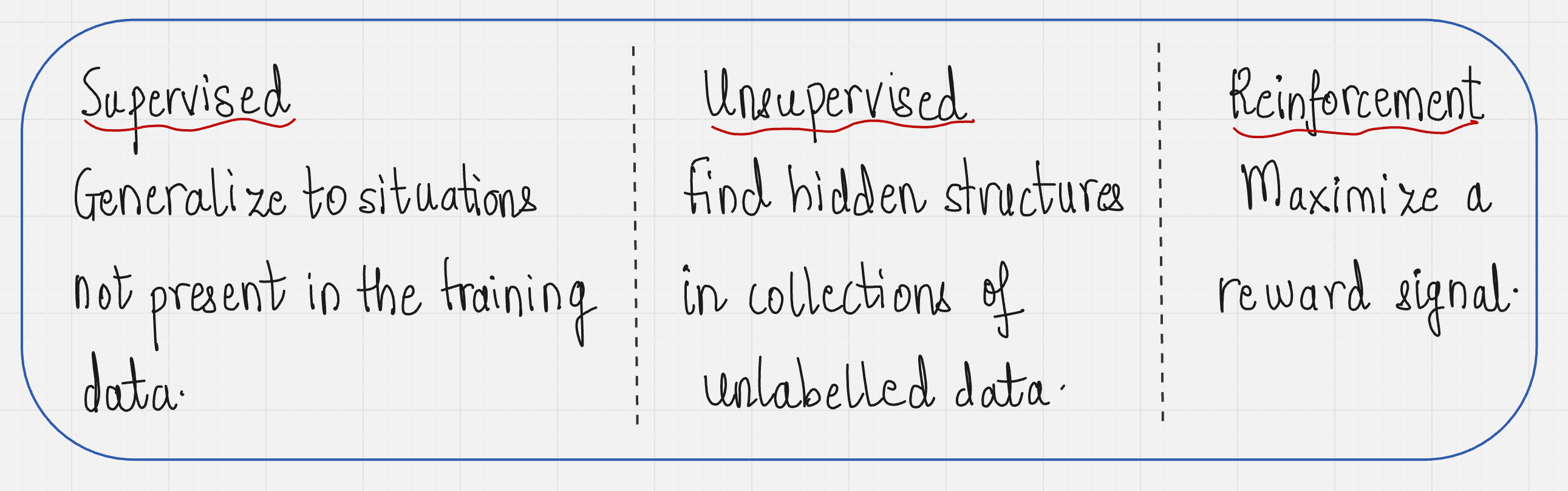
In reinforcement learning, the goal is to maximize a reward signal. These problems involve learning how to map situations to actions so as to maximize the reward signal.
Of all the forms of machine learning, reinforcement learning is the closest to the kind of learning which humans and other animals do. Many of its core algorithms were inspired from biological learning systems.
During the years 1960 to 1980, methods based on search or learning were classified as weak methods. Reinforcement learning signified a change in this way of thinking. Let us look at some real-life examples of reinforcement learning to understand it better.
The following examples have guided the development of reinforcement learning as a field:
(1) A master chess player makes a move:

The choice of the move is based on two things:
Planning by anticipating replies and counter-replies
Intuitive judgments about the desirability of moves
(2) How does a gazelle calf learn to run?
The calf struggles to get up 2-3 minutes after birth, however after 30 minutes it is seen running at 36 km/hr.
(3) How does a mobile robot make decisions?

The decision questions which the robot faces is: "Should I go to a new room in search of trash or go back to the charging station?" The decision parameters are:
Current battery charge
How much time it has taken to find the charger in the past
(4) Phil prepares his breakfast.

Actions - Walking to the cupboard, opening it, selecting a cereal box, reaching for, grasping and retrieving the box, obtaining a plate and spoon.
Each step involves a series of eye movements to obtain information and to guide reaching and locomotion. Each step is guided by goals in service of other goals with the final goal of obtaining nourishment.
What is common in all these examples?
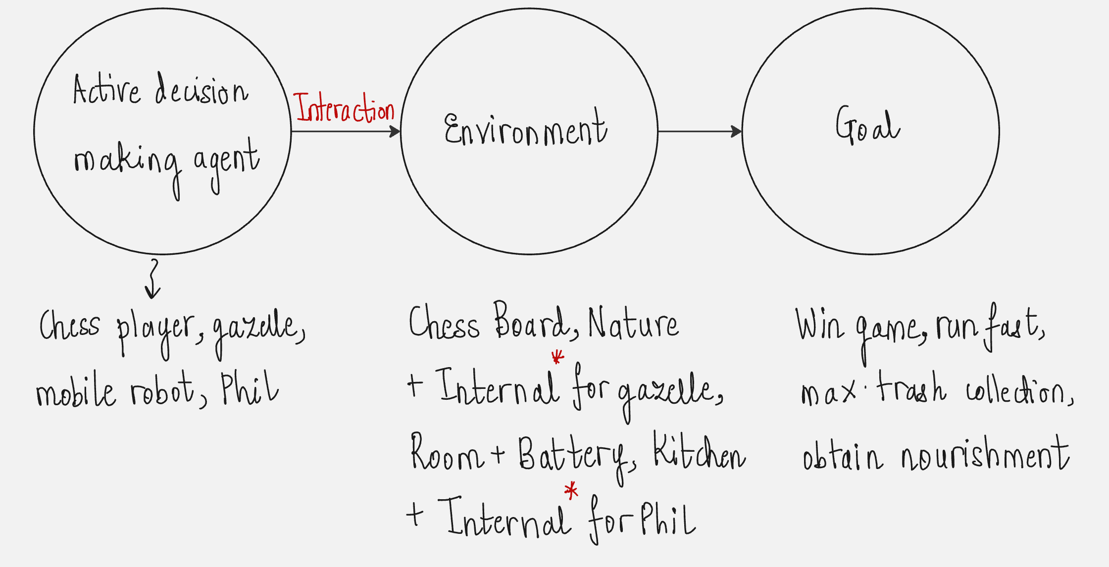
In all these examples, the agent uses its experience to improve its performance over time by interacting with the environment.
Elements of Reinforcement Learning
There are four elements of a reinforcement learning system:
(1) Policy: Informally, policy defines the agents’ way of behaving at a given time. Formally, policy is a mapping from perceived states of the environment to actions taken when in those states.
(2) Reward signal: Reward signal defines the goal in the reinforcement learning problem. At each step, the environment sends to the reinforcement learning agent a single number: reward. The sole objective of the agent is to maximize the total rewards received over time.

Reward is analogous to pleasure or pain in a biological system. If you touch a boiling vessel, your body gives you a negative reward signal.
(3) Value Function: While reward signals indicate what is good in an immediate sense, a value function specifies what is good in the long run.
Value of state is the total amount of reward the agent can expect to accumulate over the future, starting from that state.
As an example, consider a sports tournament in which there are 14 matches. Let us say a player X is selected by a team. Now in the first two matches, this player does not play well. The reward signal is low, but the captain has faith in the player and believes that he will continue to do well in later matches. Hence, even if the reward signal is low, the value is high since the long-term desirability of the player is high.
“In the field of reinforcement learning, the central role of value estimation is the most important thing that researchers learned from 1960 to 1990”
(4) Model of the Environment: Model is something which mimics the behavior of the environment. There are model-based as well as model-free methods in reinforcement learning.
Let us look at a practical example to understand the four elements of reinforcement learning.
We will look at the example of Tic-Tac-Toe.

Our goal is to construct a player which can find flaws in the opponent's play and maximize the chances of winning.
First, let us start by understanding the state, policy, and the value function.
State: Configuration of X's and O's on the 3x3 board.
Policy: Rule which tells the player what move to make for every state of the game.
Value function: For every state, we assign a number which gives the latest estimate of the probability of winning from that state. Then we draw up a table.
Have a look at the value function table drawn below.
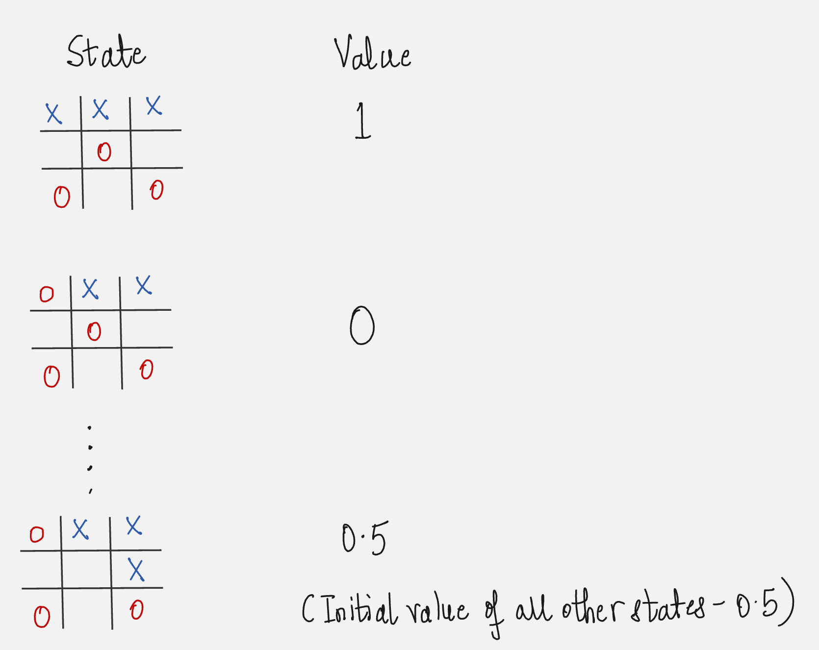
The value corresponding to the states will change as our agent plays the game more number of times.
Now, let us see how we modify the value function estimates as we play the game more number of times so that they reflect the true probabilities.
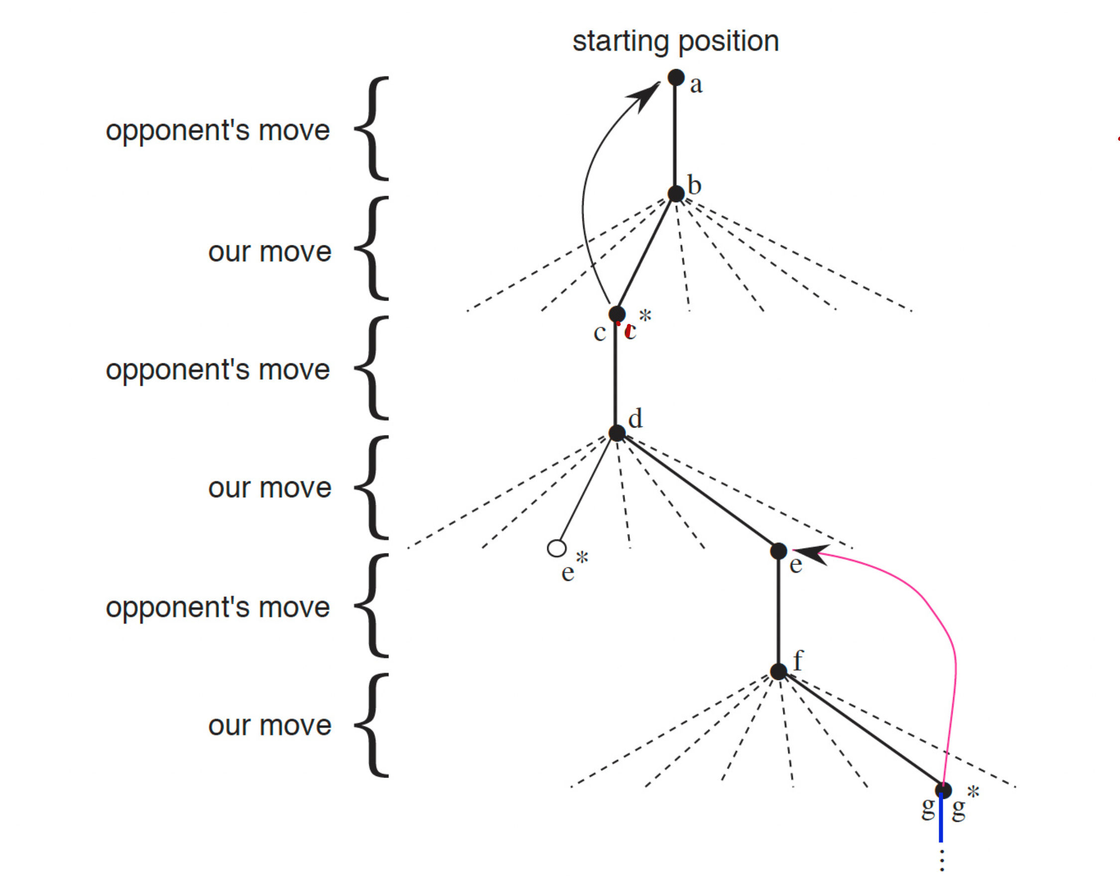
Let us say we are playing “X” and we are in the state given below:
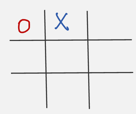
Now to play our next move, we look at all possible next states and select the one with the highest probability.
All the possible next states are given below:
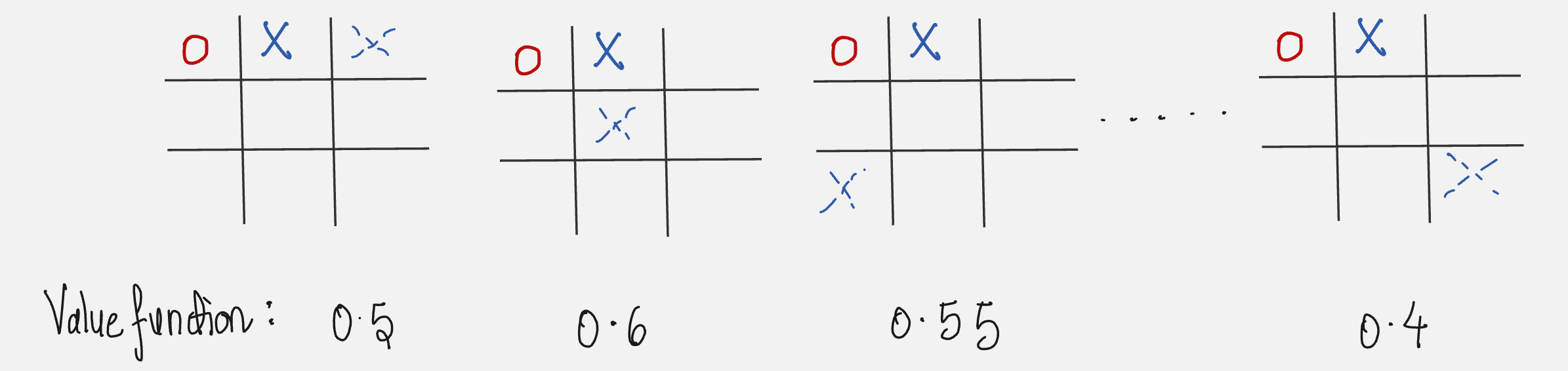
We select the move which has a value function of 0.6. This is called exploitation, selecting the state with the greatest value.
But sometimes we select randomly from the available states so that we can experience states that you otherwise might not see.
For example, we can select the state with a value function of 0.4. This is called as exploration.
While we are playing, we change the value of the states we find ourselves in. We make them more accurate estimates of the probability of winning.
After each greedy move (exploitation), the current value of the earlier state is adjusted to be closer to the value of the latter state. This is done by moving the earlier state value a fraction of a way towards the latter state. This is called backing up.
Our overall method looks as follows:
What did we learn from this example?
(1) In reinforcement learning, the learning happens by interacting with the environment/the opponent player.
(2) There is a clear goal and correct behavior includes planning, especially delayed effects of one's choices.
(3) This was an example of model-free reinforcement learning; we did not use any model of the opponent.
Several researchers have contributed to the field of classical reinforcement learning. Below is a brief history of classical reinforcement learning.
Representing a Reinforcement Learning Problem: Finite Markov Decision Processes
This problem of representing RL problems through finite Markov decision processes defines the field of reinforcement learning.
The most common framework used for representing RL problems is the Agent-Environment Interface.
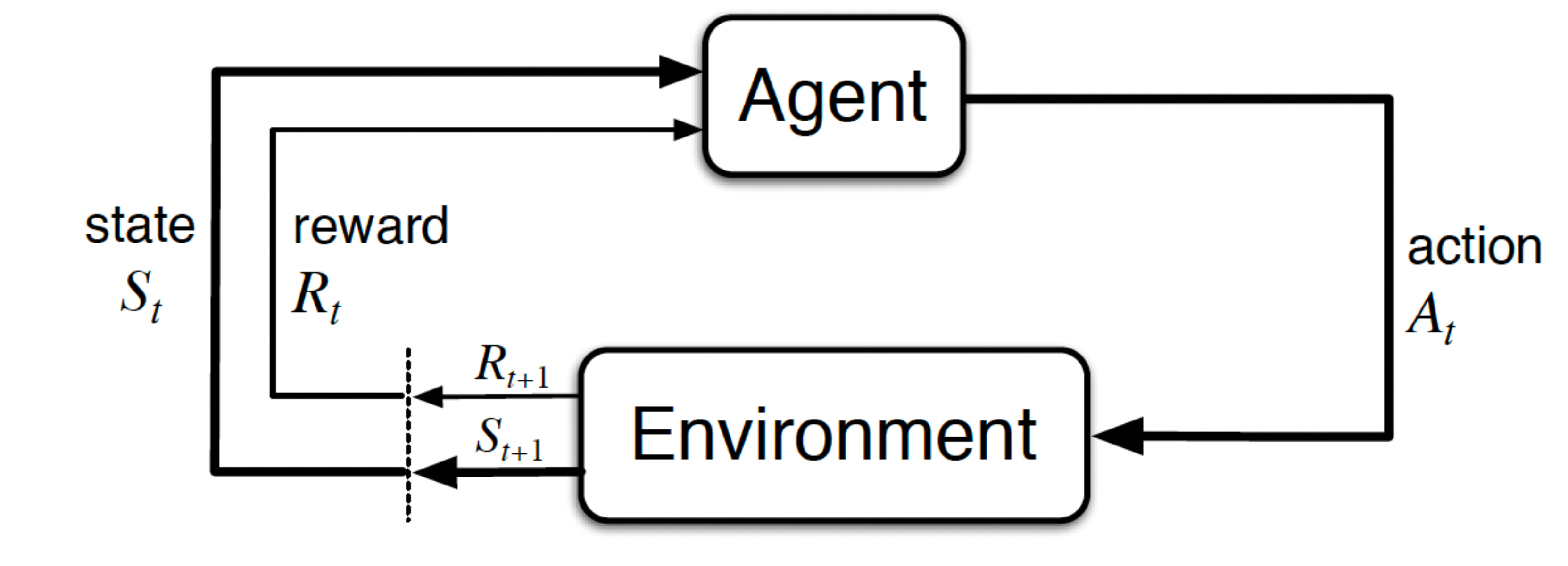
At each time step, the agent receives information on the state of the environment (also called the observation). Based on this state, the agent performs an action.
One time step later, the agent receives a reward and goes into a new state.
At each time step, the agent implements a mapping from the states to the probability of selecting each possible action. This mapping is called the agent's policy.
Examples of States: Sensor reading, chess game intermediate position.
Examples of actions:
Voltage applied to motors of robot arm
Pedaling wheels of a bicycle
Now let us look at understanding the agent-environment interface with some practical examples.
Example 1: Bioreactor
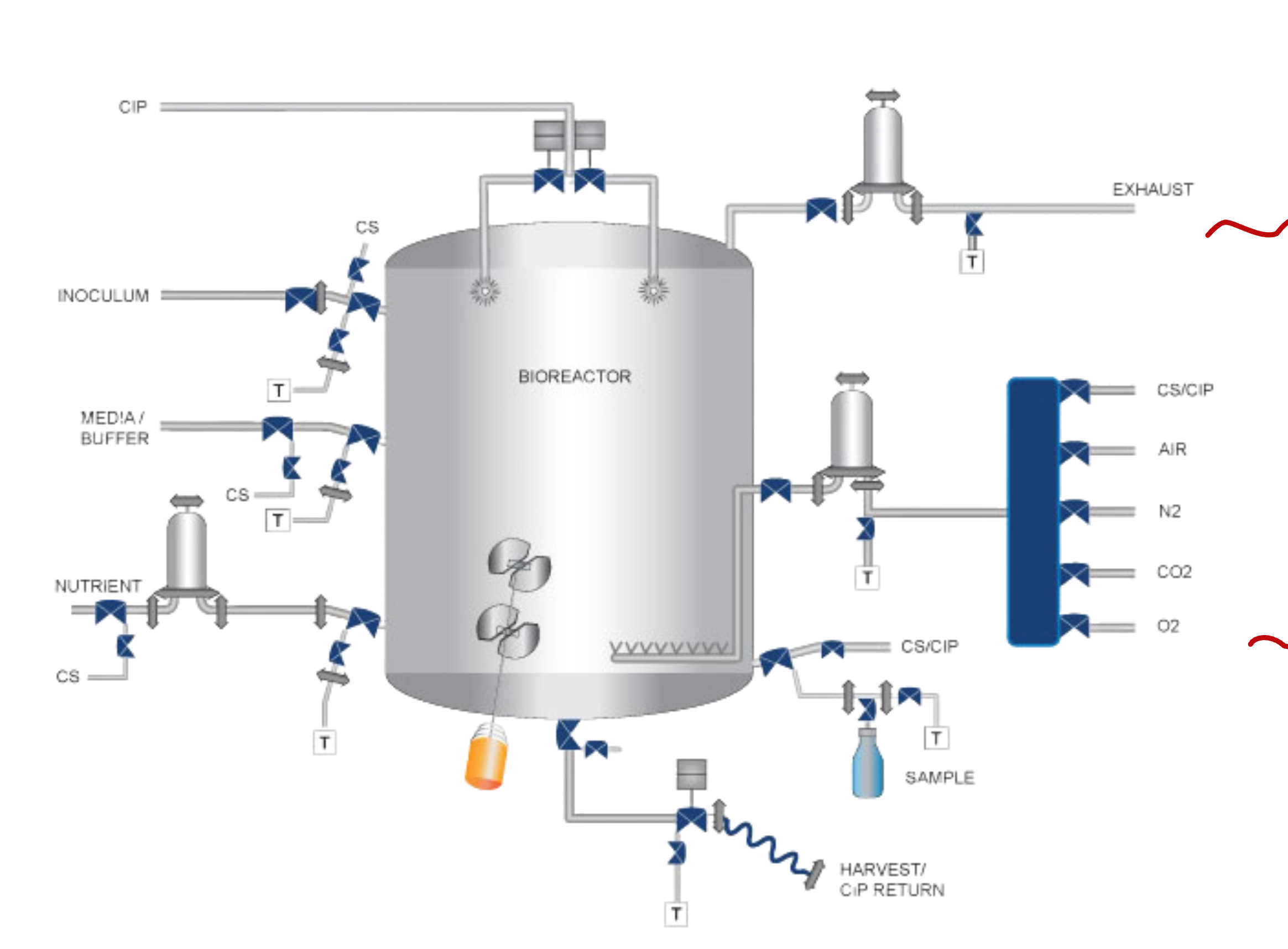
Here, the states are the sensor readings and the thermocouple readings.
The actions are:
Target Temperature: Activate Heating Element
Target Stirring Rate: Activate Motors
The rewards are the moment-to-moment measures of the rate at which useful chemicals are produced.
Example 2: Pick and Place Robot

The states are readings of joint angles and velocities.
The actions are voltage applied to motors at each joint.
The reward is +1 for each object successfully picked up and placed, and -0.02 (small negative) for jerky motion.
Now we will look at a very important section of rewards and returns.
Rewards and Returns:
The use of a reward signal to formalize the idea of a goal is one of the most distinctive features of reinforcement learning.
Let us look at some examples to understand the meaning of rewards first.
(1) Game of Chess:
Rewards are:
+1 for winning
-1 for losing
0 for a draw
(2) Robot escaping a maze:
Rewards are:
-1 for every time step that passes before the robot escapes the maze
(3) Robot collecting empty soda cans
Rewards are:
+1 for each can collected
0 for not collecting any cans
We should be careful in designing the rewards. Rewards should not be given for achieving sub-goals but only for actually attaining the final goal. Example: Giving reward in chess for taking opponent's queen.
Now let us understand the meaning of returns.
The goal of the agent is to maximize the cumulative reward it receives in the long run. We want to maximize the expected return. We can express the expected return as follows:
Here, ‘T’ denotes the final step.
This formulation is suited for applications which have a final step like a game of chess or trips through a maze. These tasks are called episodic tasks.
There are cases where the agent-environment interaction goes on continuously. These are called continuing tasks. Example, rover on a Mars expedition. For these tasks, we cannot use the above formulation.
We naturally come to the concept of discounting. Let us understand this concept using an analogy.

Rs. 100 are more valuable now compared to five years later due to inflation.
Similarly, immediate rewards are more valuable compared to rewards received later. We take this into account by saying that every reward is gamma times less valuable than the reward before, where gamma is the discounted rate, which is less than 1.
The expected return can now be written as follows:
If gamma equals 0, the agent is only concerned about immediate rewards. As gamma approaches 1, the agent considers future rewards more strongly.
Let us look at a good example to illustrate the difference between episodic and continuing tasks.
This is the classic Cart-Pole problem.
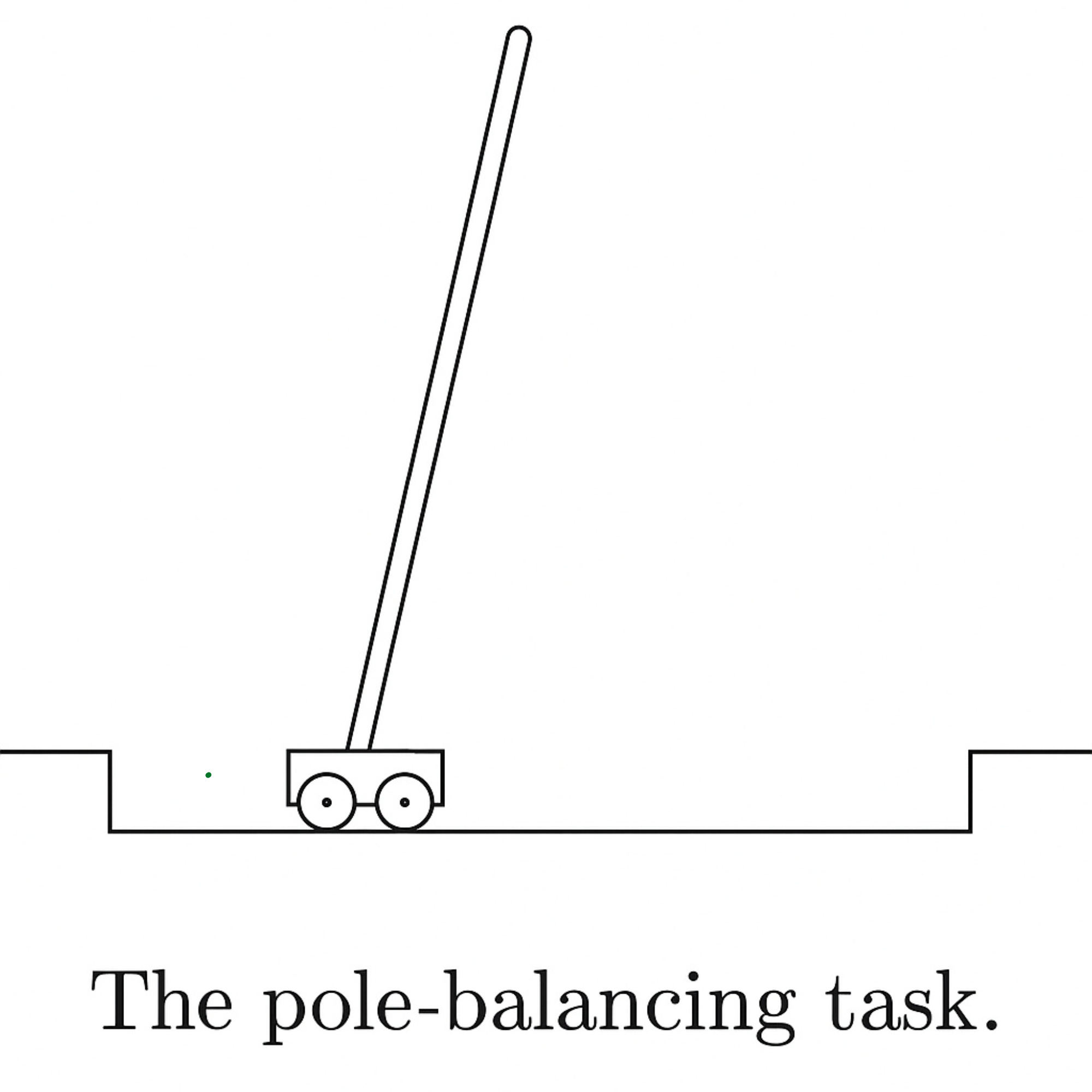
The objective is to apply forces to a car at moving along a track such that the pole does not fall over.
How would you write the rewards and returns for this problem?
Option 1: Treat the problem as an episodic task.
Reward = +1 for all time steps when the pole does not fall over, 0 for time steps when the pole does fall over.
The return can be written as follows:
Return will be maximum only if the pole does not fall over for the maximum number of time steps. This is what we want. So our reward formulation is correct.
Option 2: Treat the problem as a continuous task.
Reward = -1 for failure if pole falls, otherwise 0.
The return can be written as follows:
Return will be maximum if failure occurs very late. This is exactly what we want. So, our reward formulation is correct.
Now we move to a very important section which is the markov property.
The Markov Property:
We know that the agent makes a decision after receiving a signal from the environment. This is called a state signal. Let us look at state signals which have a specific property.
Conversations:

When we are speaking with someone, the entire history of our past conversation is known to us.
Chess:

The current configuration of chess pieces contains the entire history of past configurations.
Cannonball:

The current position and velocity of the cannonball are all that is needed to predict the next position and velocity. Past history does not matter.
What is common in all these examples?
In all of these examples, the state signals given below retain all the relevant information from the past:
Knowledge of people
Current configuration of chess pieces
Current position and velocity of cannon ball
A state signal that succeeds in maintaining all relevant information is set to a Markov or has a Markov property.
If a state signal has a Markov property, it allows us to predict the next state and the expected next state reward, given only the current state and action.
Let us look at an interesting practical example to demonstrate Markov property.
Game of Draw Poker:
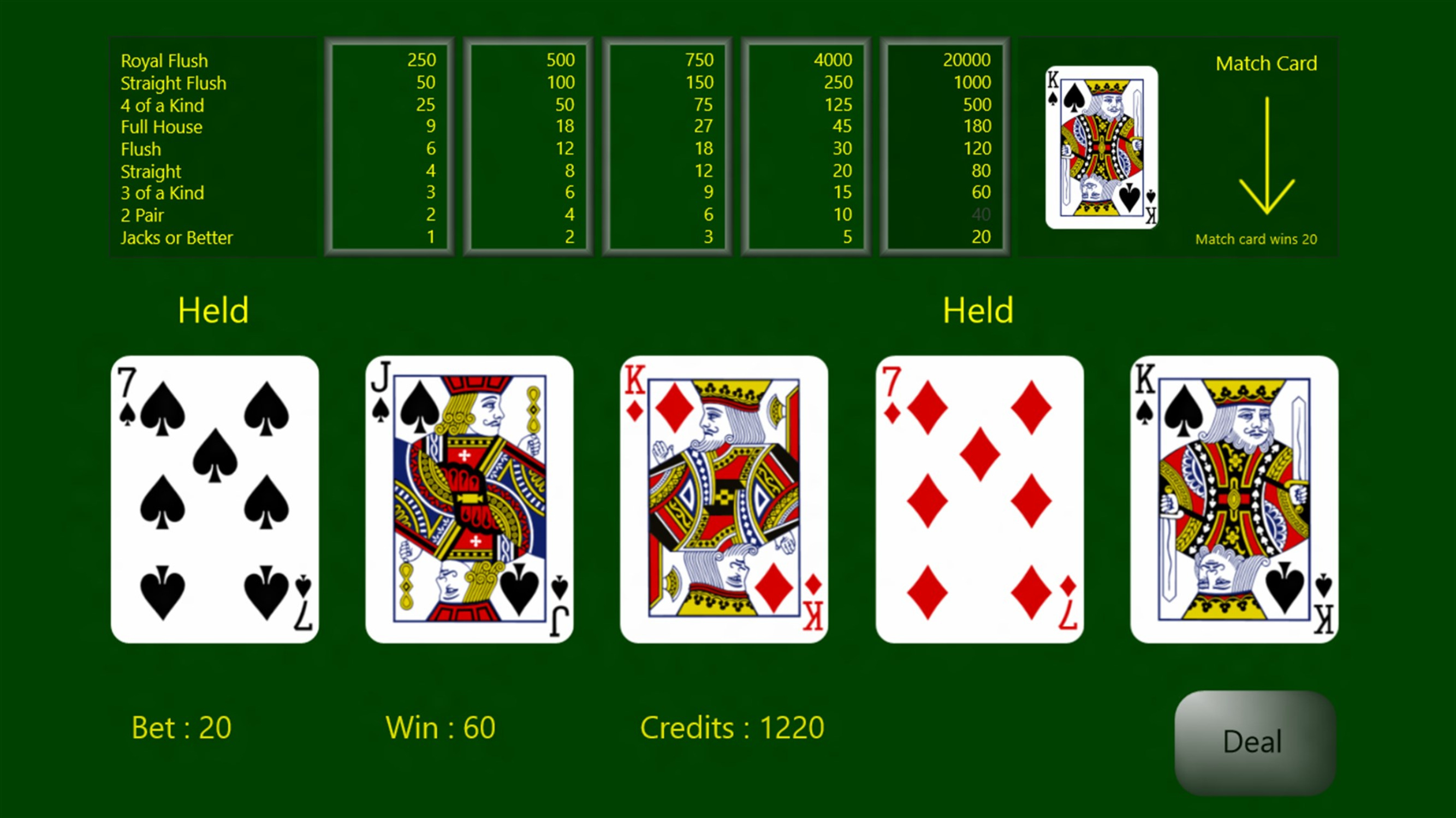
In this game, for the state to satisfy the mark of property, the player should know:
Knowledge of one's own cards
Bets made by other players
Number of cards drawn by other players
Past history with other players - Does Raj like to bluff? Does his expressions reveal something when he is bluffing?
However, no one remembers this much information while playing poker. Unless you are James Bond :)
Hence, the state representations which people use to make poker decisions are non-Markov.
Markov Decision Processes
A reinforcement learning task which satisfies the Markov property is called Markov Decision Process or MDP.
Let us look at a practical example to understand Markov decision processes.
We will look at the example of a recycling robot.

At each time step, the robot should decide on one of the following:
Whether to actively search for a can
Whether to remain stationary and wait for someone to bring the can
Whether to go back to home base and recharge the battery
The state of the robot has two possible states: High and Low
The action state of the robot has three possible actions: Wait, Search and Reward
How do we formulate the rewards?
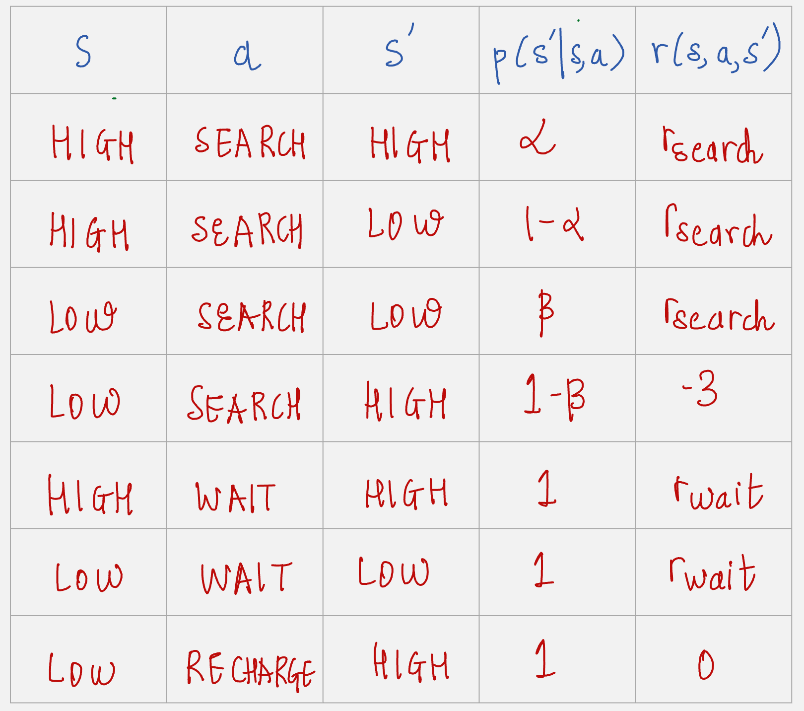
Let r_search denote the expected number of cans the robot collects while searching and r_wait denote the expected number of cans the robot receives while waiting.
So while searching the reward value will be r_search, and while waiting the reward value will be r_wait.
Reward value is -3 if the robot battery is discharged and it has to be rescued.
A period of searching starts which high energy level leaves the level high with probability alpha and reduces it to low with probability 1 - alpha.
A period of searching starts with low energy level leaves the level low with probability beta and depletes the battery with probability 1 - beta.
How can we write the transition probabilities and the expected rewards for this example? Let us build a table.
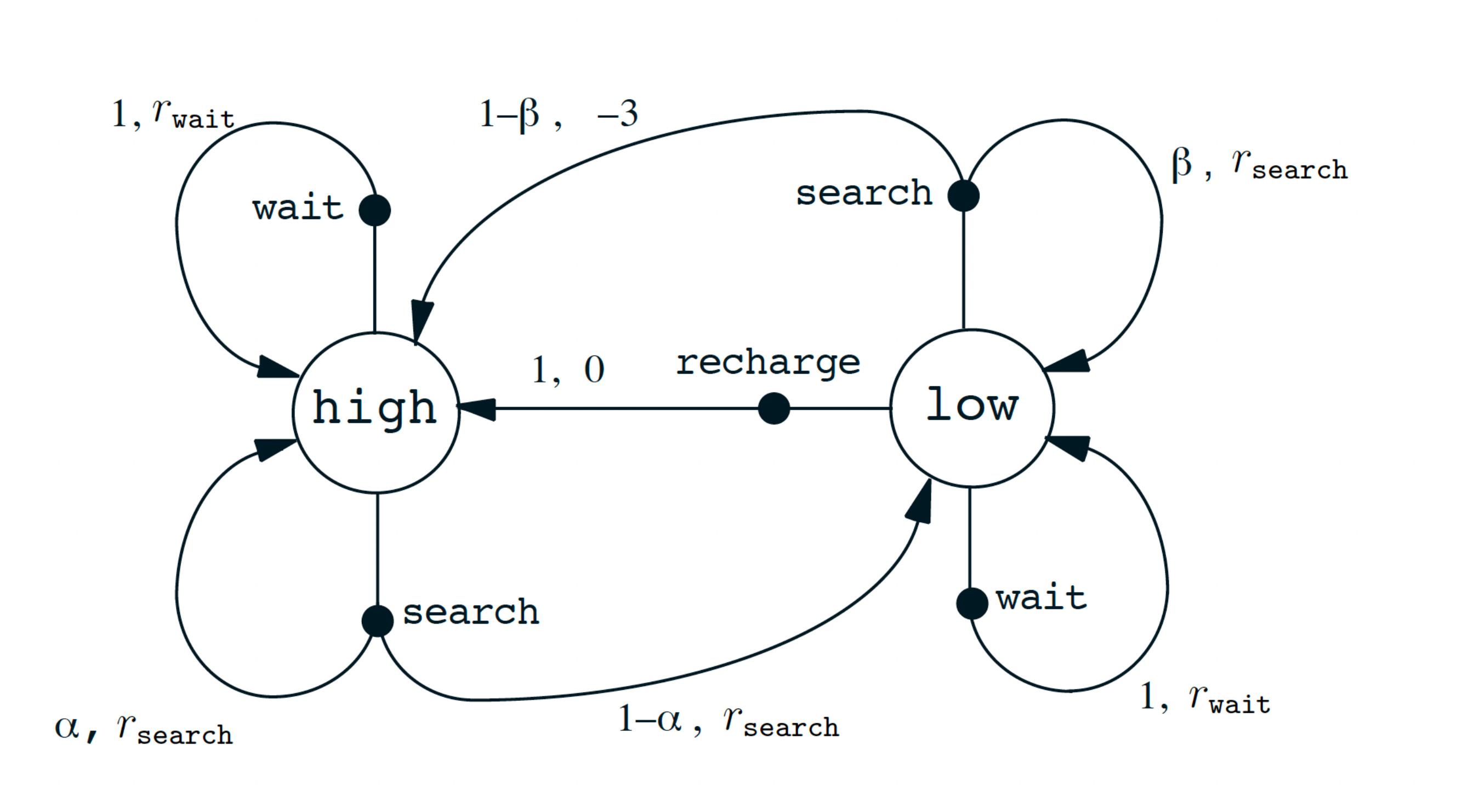
The transition graph for the recycling robot can be very nicely summarized in this figure:
Enough theory, let us look at some practical implementation now.
Reinforcement learning has always been thought of as a very theoretical field, but it's simple to implement it practically. Let us see how.

OpenAI Gymnasium
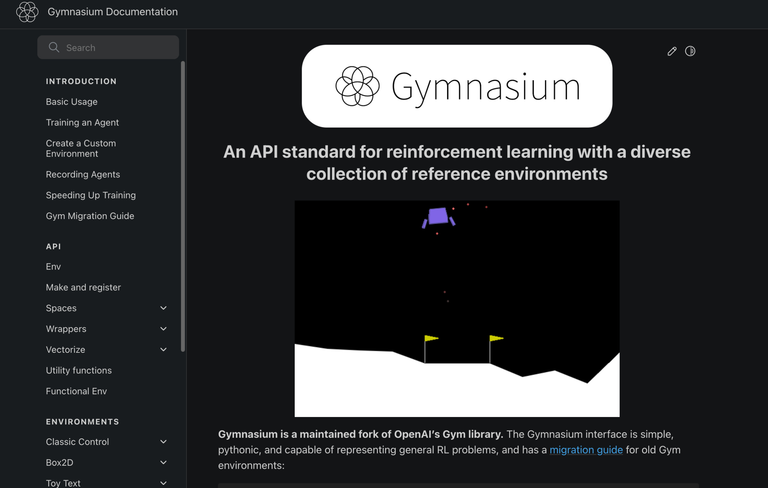
The Python library called Gym was developed by OpenAI in 2017.
In 2021, the team that developed OpenAI Gym moved the development to Gymnasium.
The main goal of Gymnasium is to provide a rich collection of RL experiments using a unified interface.
Gymnasium provides the following pieces of information and functionality:
Set of actions allowed in the environment: Discrete/Continuous
Shape and boundaries of the observations
Method called step to execute an action which returns the current observation, the reward, and a flag indicating that the episode is over
Method called reset which returns the environment to its initial state and obtains the first observation
Gymnasium has two spaces:
The action space
The environment space
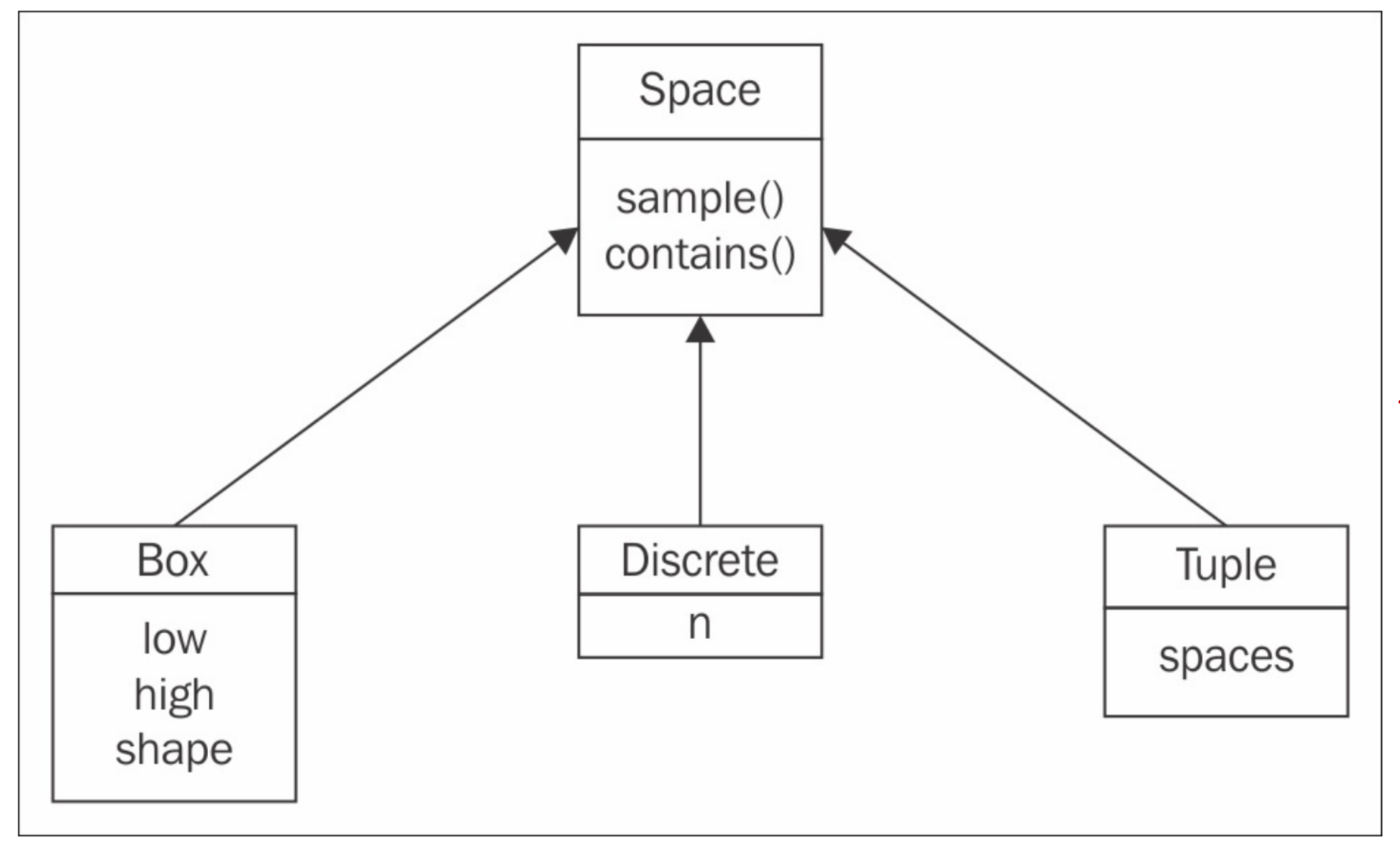
Three methods are available to create the spaces: Box, Discrete, and Tuple.
Let us look at a simple code to understand OpenAI Gymnasium better.
We will look at the Lunar Lander environment.
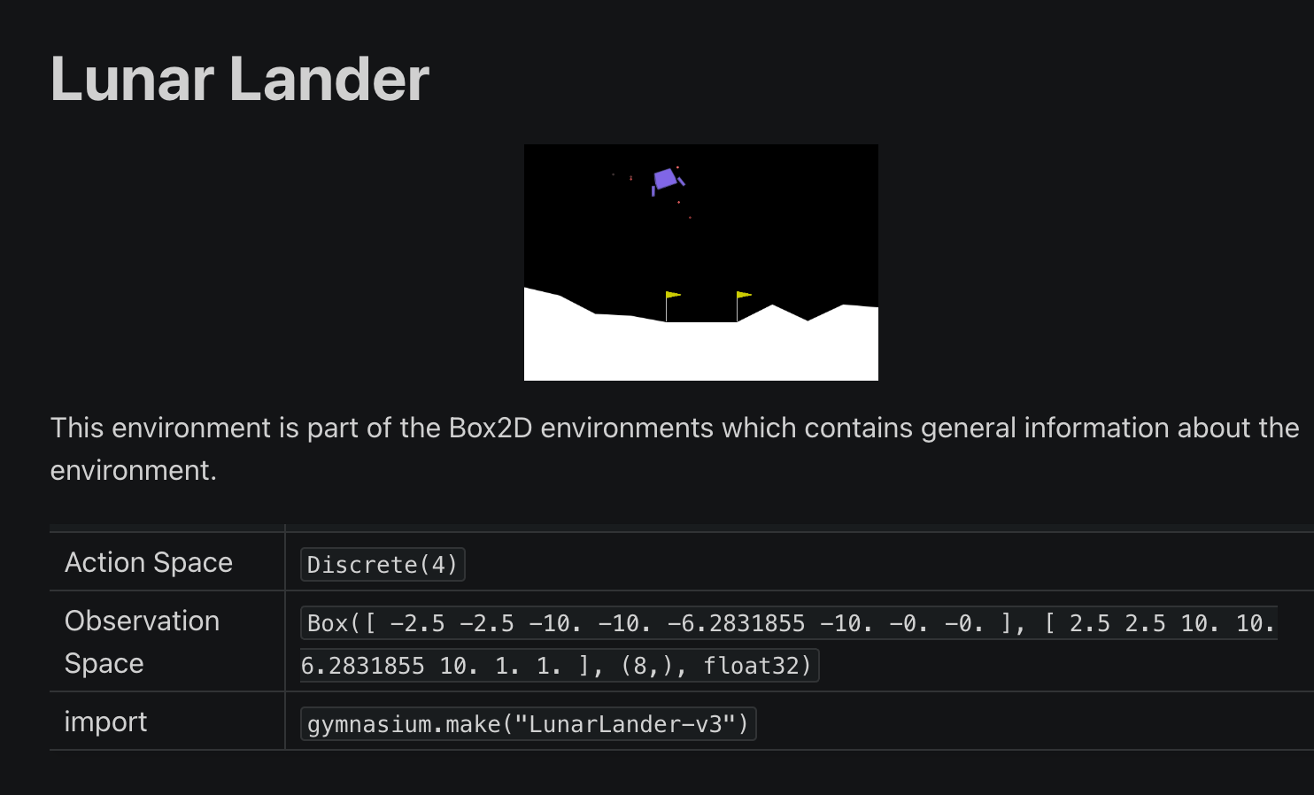
Notice how the action space and the observation space are mentioned in the environment.
The action space contains 4 actions:
Zero for doing nothing
One for firing left orientation engine
Two for firing main downward engine
Three for firing right orientation engine
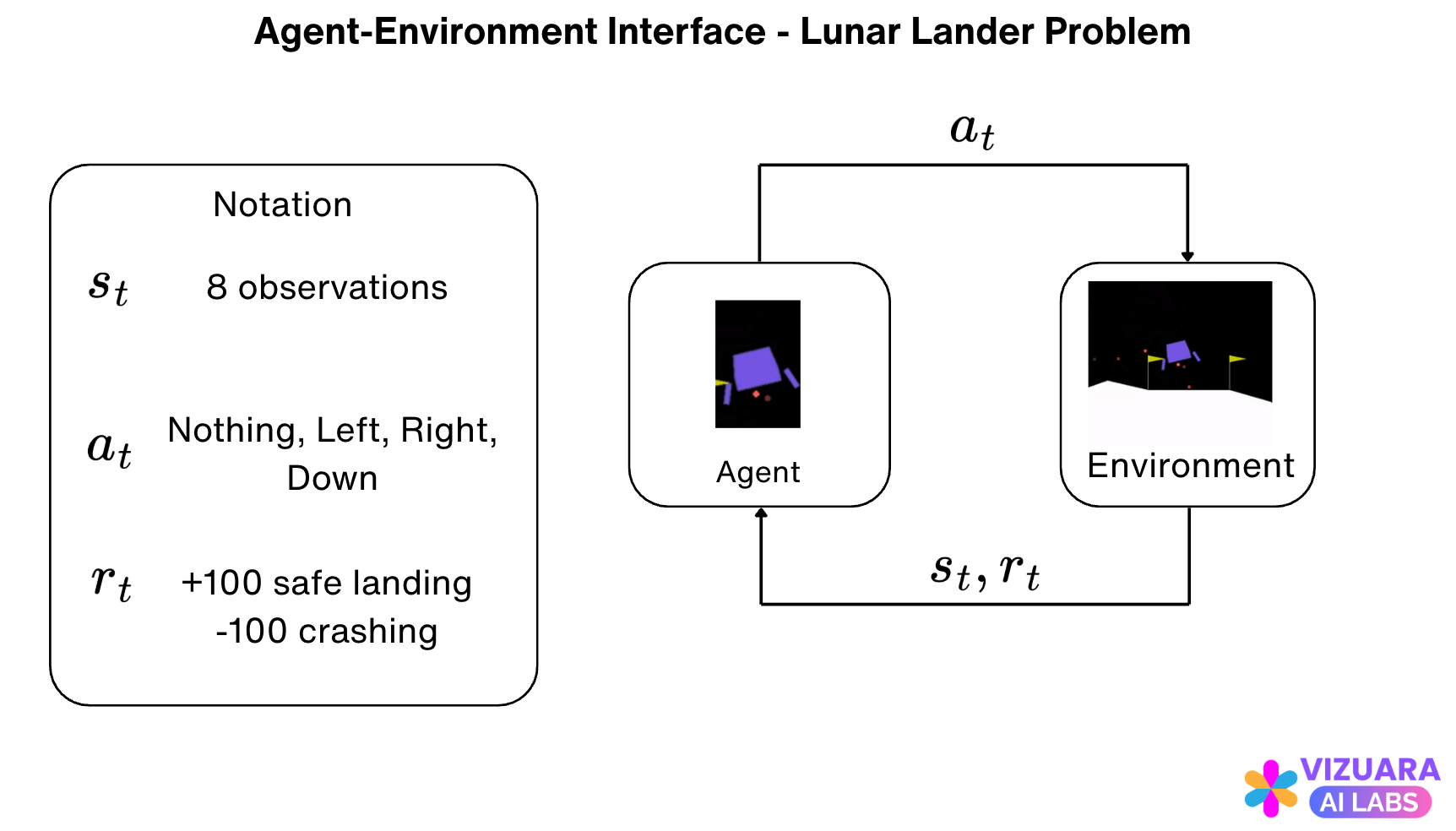
There are 8 sets of observations for:
Horizontal position
Vertical position
Horizontal speed
Vertical speed
Angle of the lander
Rotation speed
Left leg contact
Right leg contact
All these observations have a range from -infinity to +infinity.
The rewards are defined as following:
The reward is +100 for landing safely and -100 for crashing.
The reward is increased by 10 points for each leg that is in contact with the ground.
The reward is decreased by 0.03 points each frame a side engine is firing.
The reward is decreased by 0.3 points each frame the main engine is firing.
Based on these actions, observations, and rewards, here is how our agent environment interface looks like:
Now let's look at our first code to create a sample from the observation and action spaces.
First, let us look at the dependencies you need to install for this.
pip install gymnasium[box2d] - That’s All!
import gymnasium as gym

# Create the environment
env = gym.make("LunarLander-v3")

# Sample an action
sample_action = env.action_space.sample()
print("Sample action from action space:", sample_action)

# Sample an observation
sample_observation = env.observation_space.sample()
print("Sample observation from observation space:", sample_observation)

# Optional: check the space definitions
print("Action space:", env.action_space)
print("Observation space:", env.observation_space)

env.close()
This code will give you a sample action from the action space and from the observation space as well. There are three functions that we see here:
The gym.make( ) function creates the environment for us.
The env.observation_space.sample( ) samples an observation from the observation. space.
The env.action_space.sample( ) equals an action from the action space.
You might be thinking that, but I never defined the action space and the observation space. They are defined in the environment for you.
Now let us control our lunar lander.
The following is a code for controlling your lunar lander with random actions. Remember that we are not using any policy right now.
import gymnasium as gym

# Create the environment
env = gym.make("LunarLander-v3", render_mode="human")

env.reset()

for step in range(200):
    env.render()
    env.step(env.action_space.sample())

env.close()
Let us understand this code in detail.
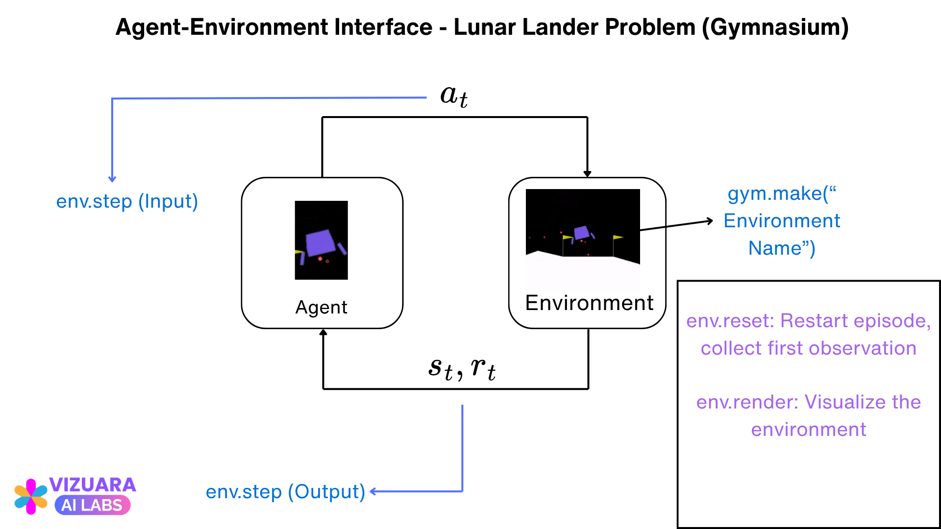
The first step is the creation of our environment using the gym.make( ) function.
Next we have `env.reset( )`, which is used to reset the episode for episodic tasks (remember we talked about episodic tasks before), and also collect the first observation from the environment. This is a mandatory command.
The env.step( ) function takes the action as the input and gives the following as the output:
(1) Observation - This represents the agent's observation of the environment after taking the action. For example, in a classic control environment like Cart-Pole, it might be a NumPy array containing positions and velocities.
(2) Reward - This represents the amount of reward received as a result of taking the action. The scale and the meaning of reward are environment-specific.
(3) Terminated - A Boolean indicating whether a terminal state has been reached or not. If true, the episode has ended because the task was completed or failed.
(4) Truncated - A Boolean indicating whether a truncation condition has been satisfied. This typically signifies that the episode has ended prematurely, often due to a time limit or agent going out of bounds (I have personally not understood the requirement of this, but I am just explaining it here anyways.)
(5) Info - A dictionary containing diagnostic information useful for debugging and analysis.
Let us understand all this by referring to our agent-environment interface diagram which we looked at before.
Once you run this code, you should see a py game window open with the lunar rover moving towards the landing surface.
You might be wondering that: well, this is not very good. Our lunar lander just falls off - it is not oriented properly towards the end.

If only it was this easy to run reinforcement learning problems :)
To understand why we are not doing good, go back and check the 4 elements of reinforcement learning problems. We have missed a major element here.
Yes, the policy.
We will cover this in detail in the subsequent lectures.
For now, play around with Gymnasium and try various environments.
See you next time!