Policy Gradient Methods in Reinforcement Learning

So far, our policy estimation has been defined based on the following rule: For every state, look at the action value function Q and ask the question: which action is giving me the maximum Q value?

But doesn't this feel like an indirect method of estimating the policy? It is like finding “A” by first estimating “B” and then using “B” to find “A”.

In this article, we are going to look at a class of methods which can be used to directly find “A”.

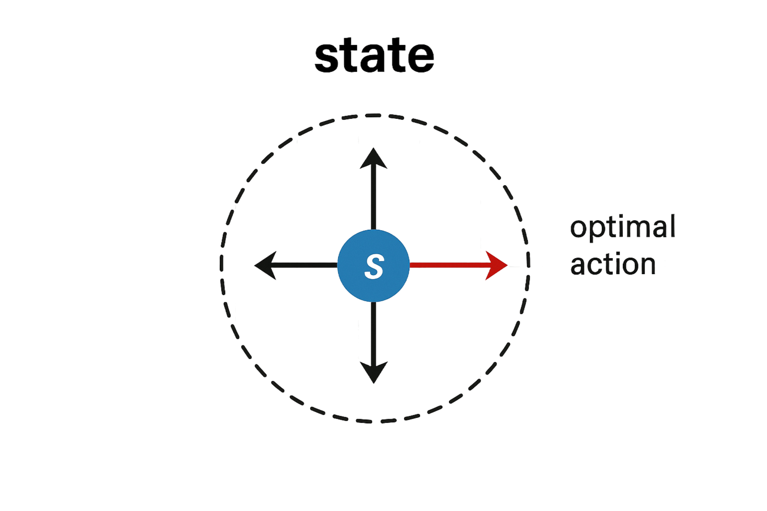
Remember that the policy is defined by π(a|s), which means the probability of picking action “a” while in state “s”.

The question we are asking in this article is: Can we directly estimate π(a|s) to predict the probabilities of all possible actions for a given state?

Now we introduce a policy parameter θ and write the policy as π(a|s, θ). In general, θ belongs to a D-dimensional space, θ ∈ ℝ^D.

Let us look at policy parameterization now.

Policy Parameterization:

How do we parameterize the policy?

Let us say for a state S there are five possible actions. We write the numerical preferences for these actions as follows:

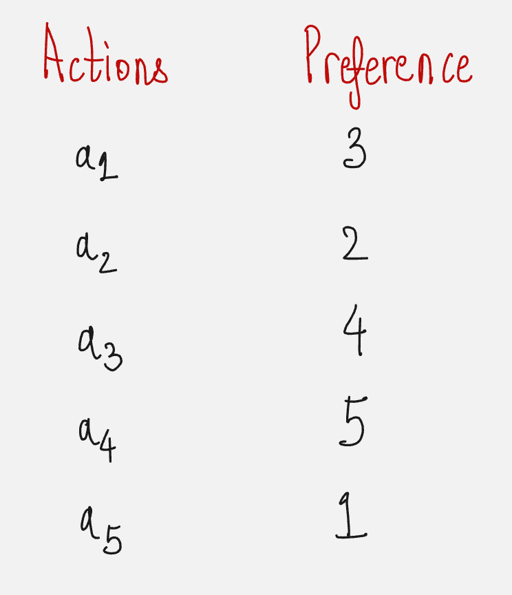
The above can be captured in a functional form denoted by h(a, θ).

If we assume h(a, θ) to be a polynomial, then we can capture the preferences as follows:

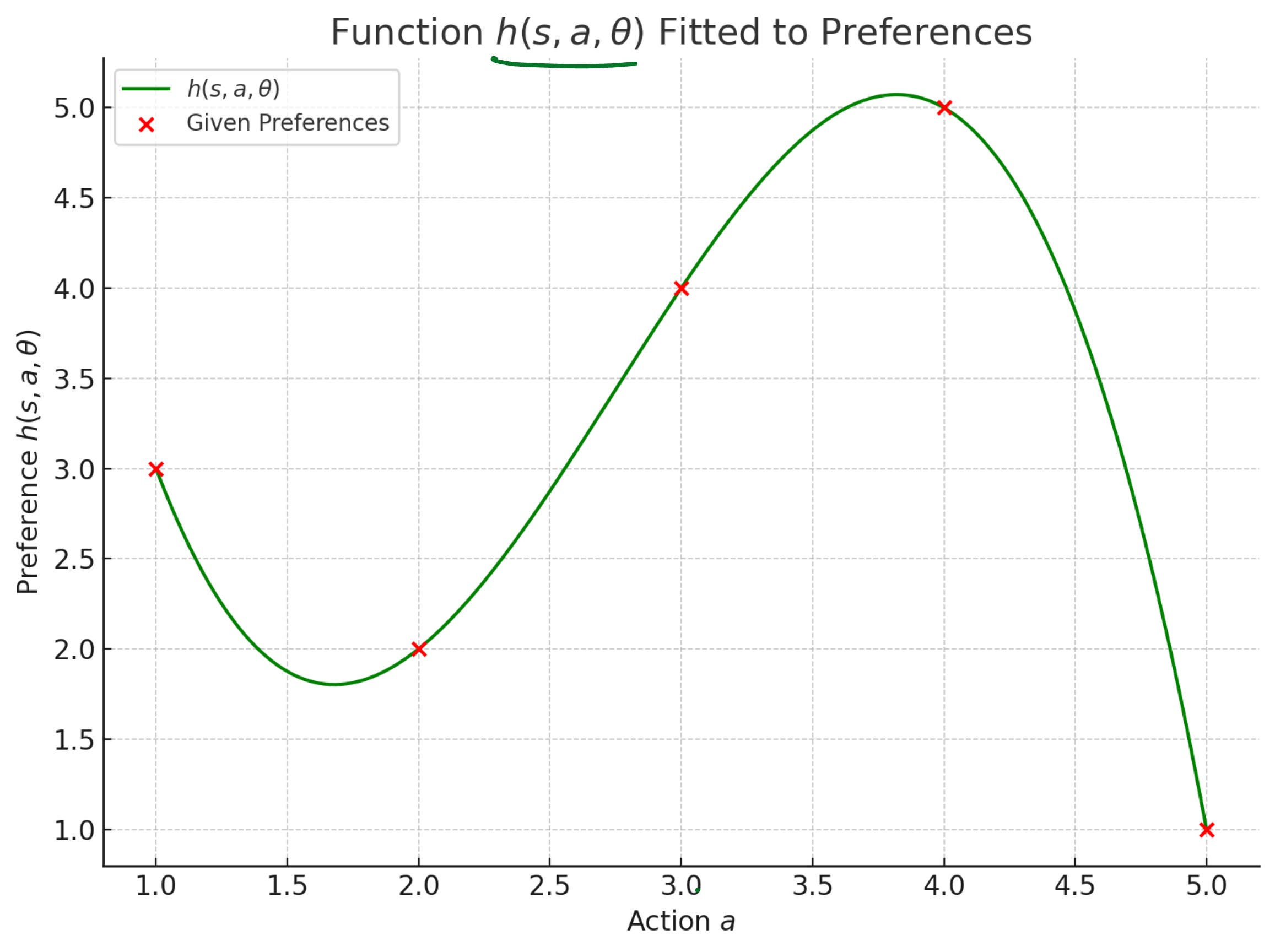
Note that here the polynomial is written in terms of the policy parameter θ. It can assume a functional form like this:

\(h(a,\theta) = \theta_{0} + \theta_{1}a + \theta_{2}a^{2}\)

The policy parameter is a vector of three values and it represents something like “weights” which have to be tuned to match the preferences.

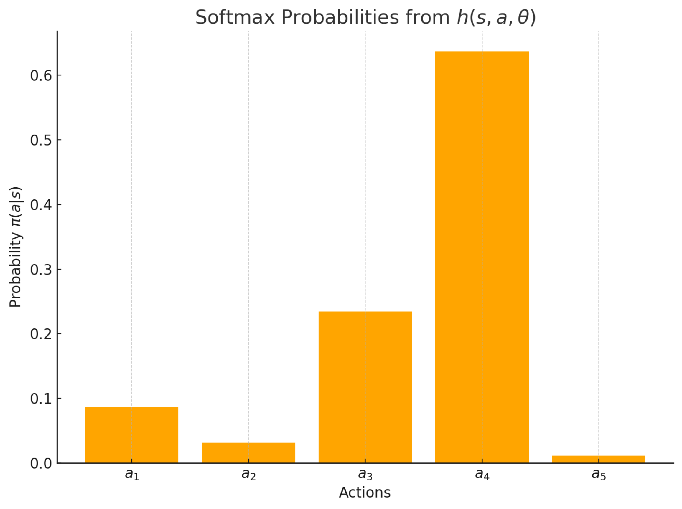
Now the question is, how do we convert the preferences into probabilities? Remember that our policy will predict the probabilities of all the possible actions.

We can simply use the softmax function to convert the references to probabilities. The conversion formula looks as follows:

\(\pi(a|s,\theta) = \frac{e^{h(a,\theta)}}{\sum e^{h(a,\theta)}}\)

The probabilities for all the actions based on the preferences look as follows:

Fun Fact: h(a, θ) was a deep neural network when AlphaGo bet the human Go champion.

One of the fundamental tasks in policy gradient methods is to train our policy to find the values of the policy parameters by training our policy to maximize the performance measure.

But what exactly is this performance measure? Let us understand.

Performance Measure

Our objective is to maximize something which captures the performance of our policy parameter.

This something is called a performance measure and is denoted by J(θ).

The whole objective of the Reinforcement Learning process is to optimize the cumulative rewards received in the entire episode.

This is exactly what the value function captures.

Hence, in policy gradient methods, there is a standard performance measure used throughout the literature, which is the value function of the initial state of the episode. This is denoted by V(s₀)

Let us look at a sample curve for the performance measure (value function of the initial state) as follows:

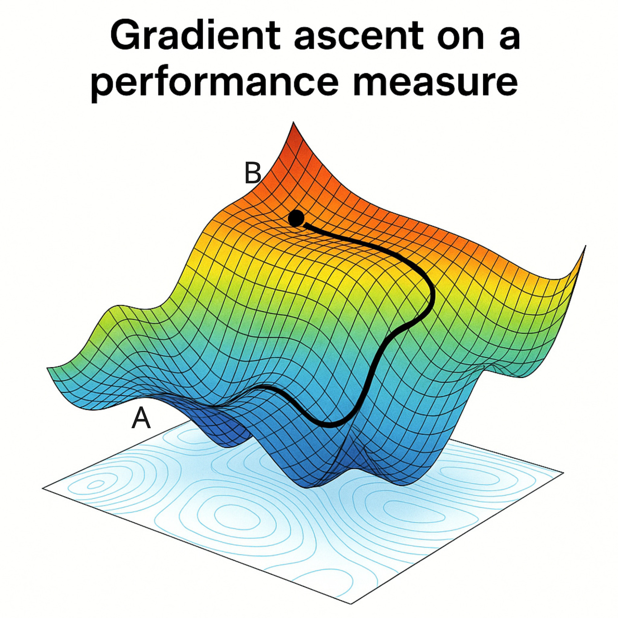
If we have the performance measure with us and we are starting from point A, then we want to slowly move upwards this curve and reach point B.

You might have seen something like this before.

Yes, this is very similar to the gradient descent algorithm in machine learning. The only difference here is that since we are maximizing our objective, we are performing an ascent instead of a descent.

The policy parameter update rule is then given according to the gradient ascent formula as follows:

\(\theta_{t+1} = \theta_{t} + \alpha\nabla_{\theta} J(\theta)\)

So you can see from the above formula that once we understand how to climb the mountain, we will be able to successfully update our policy parameters.

But to climb the mountain, we need to find out, for every step taken in the policy parameter direction, how much will the performance measure changes by.

How will we find this? How will we find the gradient of the performance measure?

Finding the gradient of the performance measure

We are going to do a small derivation right now through which you will understand how this gradient is calculated.

We are going to perform this derivation in multiple steps.

Step 1: Substituting value function in the performance measure

\(\nabla J(\theta) = \nabla E_{\tau \sim \pi_{\theta}} [G(\tau)]\)

Here, τ signifies the trajectories and G is the return for each trajectory. It is important to understand that the trajectory is not fixed and for the same policy, we can have multiple different trajectories because the policy output is probabilistic in nature, it is a deterministic policy.

Step 2: Expanding the Expectation

\(\nabla J(\theta) = \nabla \int P(\tau|\theta)G(\tau)\)

Here, P denotes the probability of sampling a specific trajectory from all possible trajectories for the given policy.

Step 3: Bring Gradient under Integral

\(\nabla J(\theta) = \int \nabla P(\tau|\theta)G(\tau)\)

The above equation simply comes from this rule: The gradient of a sum is equal to the sum of gradients.

Step 4: Log-Derivative Trick

\(\nabla J(\theta) = \int P(\tau|\theta) \nabla \text{log} P(\tau|\theta) G(\tau)\)

The above equation comes from this rule: The gradient of the log of a function is equal to the gradient of the function divided by the function itself.

Step 5: Return to Expectation Form

\(\nabla J(\theta) = E_{\tau \sim \pi_{\theta}}[ \nabla \text{log} P(\tau|\theta) G(\tau)]\)

Step 6: Expanding the Probability

Now I am going to list down a series of steps which might be slightly hard to comprehend. However, if you go through it properly, you will be able to understand:

Brace yourselves!

\(P(\tau|\theta) = \rho_{0}(s_{0}) \prod_{t=0}^{T-1} P(s_{t+1}|s_{t},a_{t})\pi(a_{t}|s_{t}) \)

\(\nabla \text{log} P(\tau|\theta) = \nabla \text{log} \rho_{0}(s_{0}) + \sum_{t=0}^{T} \nabla \text{log} P(s_{t+1}|s_{t},a_{t}) + \sum_{t=0}^{T} \nabla \text {log} \pi (a_{t}|s_{t})\)

In the above expression, the first term and second term are 0, since they do not depend on θ.

So, we get:

\(\nabla \text{log} P(\tau|\theta) = \sum_{t=0}^{T} \nabla \text {log} \pi (a_{t}|s_{t})\)

Step 7: Final Expression

\(\nabla J(\theta) = E_{\tau \sim \pi_{\theta}}[\sum_{t=0}^{T} \nabla \text {log} \pi (a_{t}|s_{t})G(\tau)]\)

The gradient of the performance measure of the policy is given by the expected value over all the possible trajectories of the summation of the grad-log action probabilities for each trajectory times the reward received at the end of the trajectory

The above equation is the single most important equation to understand policy gradient methods.

The above equation is very closely linked with the policy gradient theorem.

The first proof for the Policy Gradient theorem came about in 1999.

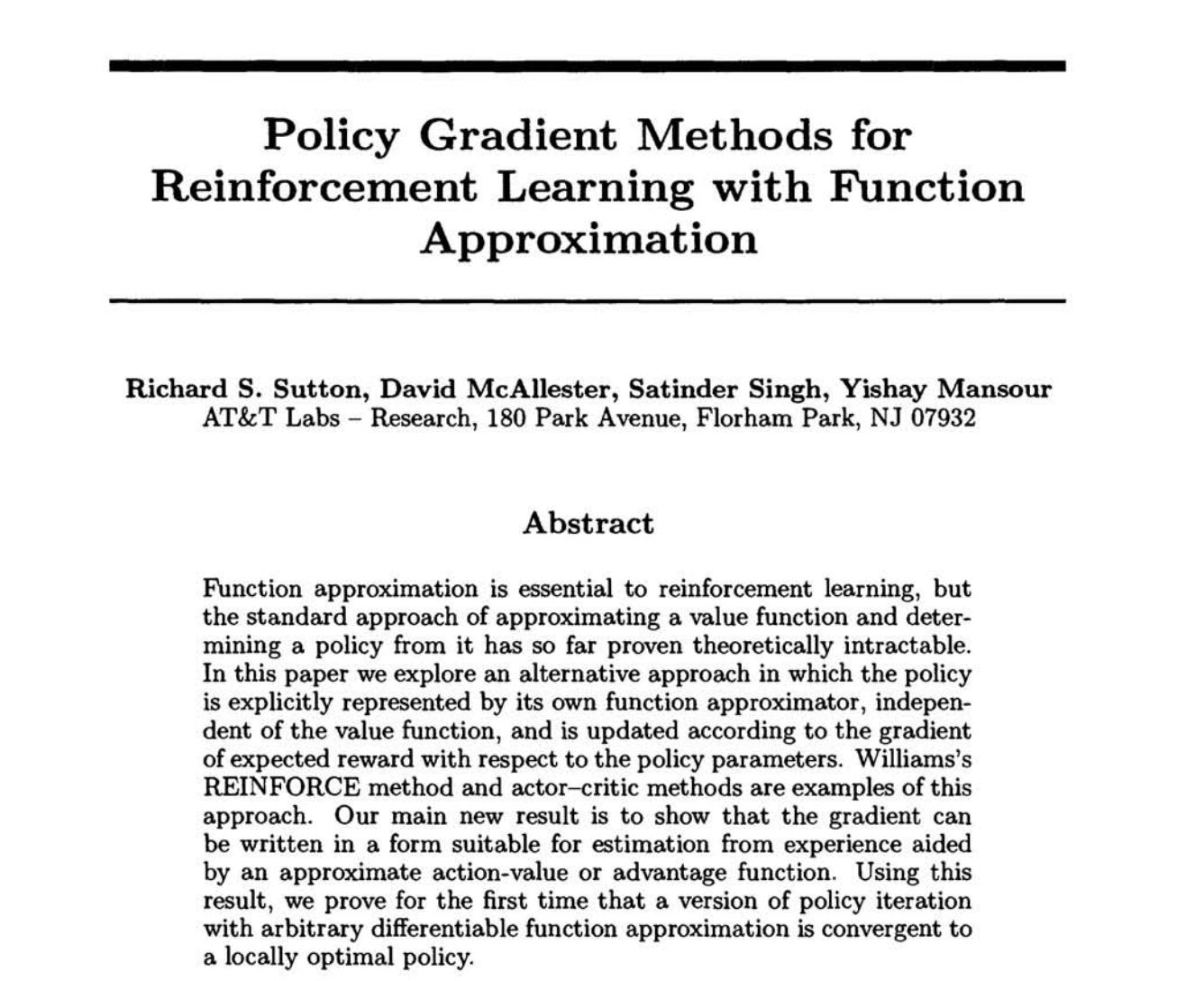
The study was performed in Richard Sutton’s group, who is one of the pioneers in the field.

Now let us try to understand the intuition behind this equation and what does it really say.

Intuition behind gradient of the performance measure

Let us say that we have an old policy (O). We take one step in the environment and we collect the reward. Now we want to update the policy based on this step that we have taken in the environment.

The new policy is denoted by N.

Using the formula for the gradient of the performance measure, we can find the direction in which we want to move to improve our performance measure.

It would look something as follows:

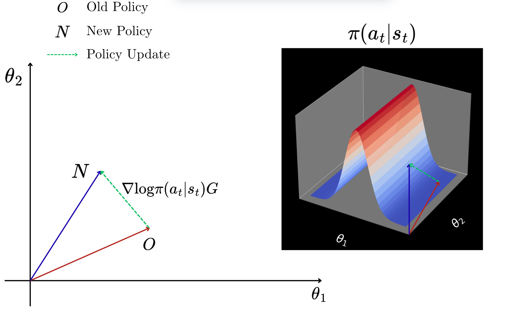
Now, from this diagram, what we can see is that when we are updating the policy, we are also moving along the policy curve as shown on the right of the above figure.

So if we have a return which is very good, then we are going to take longer steps in the curve, moving towards the peak of the mountain, which means that we are going to increase the probability of taking the specific action a_t for the given state s_t.

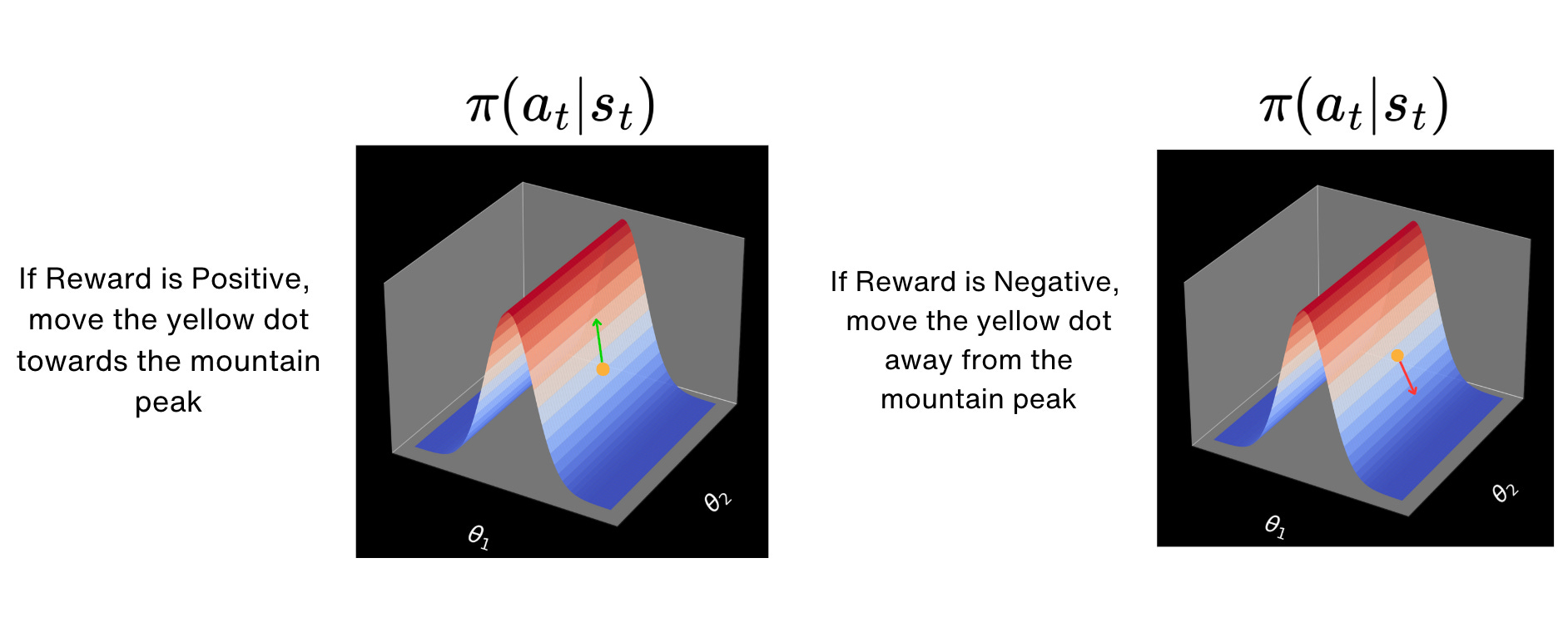
Similarly, if we have a return which is close to zero or negative, then we are going to take steps which move us away from the peak of the mountain. This means that we are going to decrease the probability of taking the specific action a_t for the given state s_t.

Because actions which give good returns are reinforced and actions which give bad returns are penalized, this is called as the REINFORCE algorithm.

REINFORCE Algorithm:

\(\nabla J(\theta) = E_{\tau \sim \pi_{\theta}}[\sum_{t=0}^{T} \nabla \text {log} \pi (a_{t}|s_{t})G(\tau)]\)

Problems with the REINFORCE Algorithm

Imagine that you want to find out the average age of your country. You go ahead, collect a lot of samples, and find out the average.

Your estimate is going to heavily depend on which people you did sample. For example, if you only sample people above 60 years of age, you will wrongly think that the average age of the country is more than 60.

From the above graph, we can see that the true population (shown in blue) is very different from all the three sample distributions.

So then, how do we select the correct sample? Which is the true distribution?

This is exactly the problem with the REINFORCE method.

Because we are sampling from a lot of trajectories and calculating the expected value, the main issue with REINFORCE algorithm is that of variance.

To solve this problem, people have modified the REINFORCE method with something called REINFORCE with baseline.

REINFORCE with Baseline

In the REINFORCE with Baseline method, a constant value is subtracted from the return. This constant value is dependent on the state.

This makes sure that states with high return values do not end up influencing the policy parameter update.

This constant value is called the baseline.

The gradient of the performance measure is updated as follows:

\(\nabla J(\theta) = E_{\tau \sim \pi_{\theta}}[\sum_{t=0}^{T} \nabla \text {log} \pi (a_{t}|s_{t})(G(\tau) - b(s))]\)

Here, b(s) represents the baseline.

Another small change people make is that they replace the total episode return with the return obtained from that state.

Hence, the updated gradient of the performance measure is given as follows:

\(\nabla J(\theta) = E_{\tau \sim \pi_{\theta}}[\sum_{t=0}^{T} \nabla \text {log} \pi (a_{t}|s_{t})(G(t) - b(s))]\)

A common practice is to use the value function itself as the baseline.

This method is also called the Actor-Critic method since the value function is like the critic which evaluates the actor which is the return.

Now let us implement these methods for a practical problem so that we can understand their implementation is much better.

POLICY GRADIENT METHODS FOR CARTPOLE PROBLEM

We will take the example of a cart pole problem. This environment is available on OpenAI Gymnasium. It allows us to study the policy gradient methods.

There are only two actions in the cart pole problem: left or right. Our main objective is to move the cart in such a way that it does not fall over for a long time.

The overall workflow for solving this problem using the policy gradient methods looks like follows:

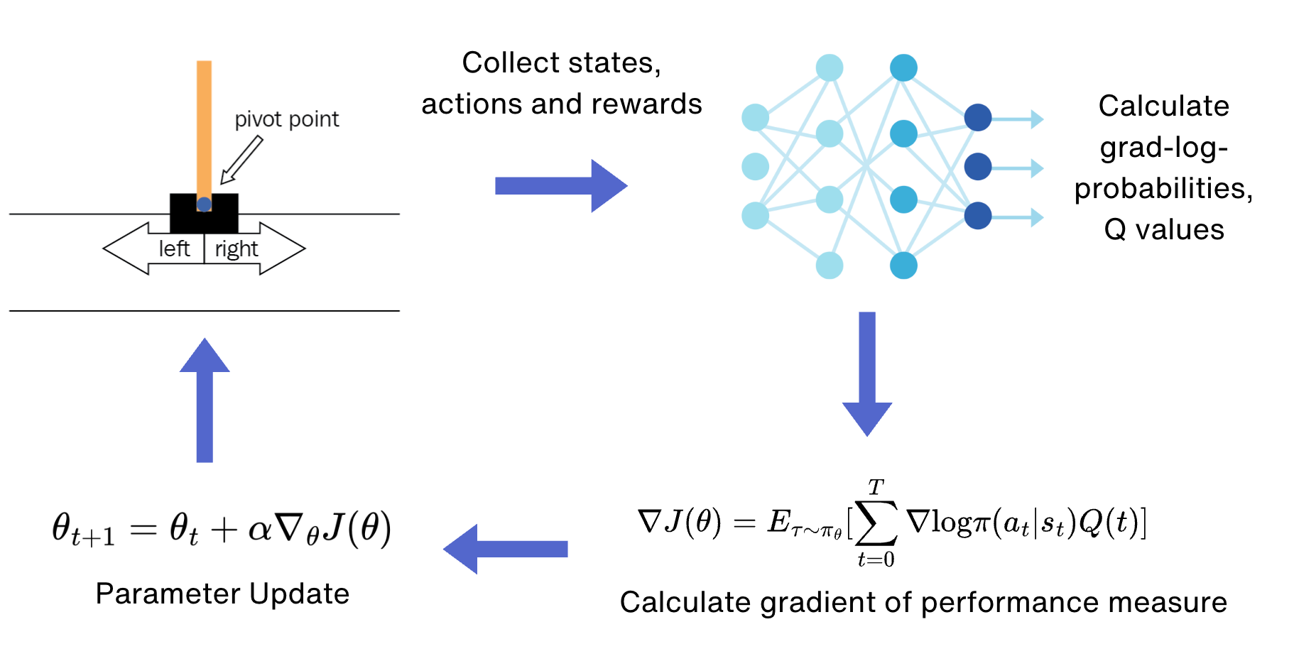
Step 1: Defining the policy neural network

Our policy neural network will have three layers:

1. An input layer

2. A hidden layer with 128 neurons

3. An output layer

We will use a ReLU activation function.

The following is the piece of code which we will use to define our neural network:

class PGN(nn.Module):
    """
    Policy Gradient Network
    """
    def __init__(self, input_size: int, n_actions: int):
        super(PGN, self).__init__()
        self.net = nn.Sequential(
            nn.Linear(input_size, 128),
            nn.ReLU(),
            nn.Linear(128, n_actions)
        )

    def forward(self, x: torch.Tensor) -> torch.Tensor:
        return self.net(x)

Step 2: Defining a function to calculate the Q-values

We need to define a function to estimate the Q-values based on the rewards which we will collect in the future.

This function will be defined using the following piece of code:

def calc_qvals(rewards: tt.List[float]) -> tt.List[float]:
    """
    Calculates discounted rewards for an episode.
    Args:
        rewards: A list of rewards obtained during one episode.
    Returns:
        A list of discounted total rewards (Q-values).
    """
    res = []
    sum_r = 0.0
    for r in reversed(rewards):
        sum_r *= GAMMA
        sum_r += r
        res.append(sum_r)
    # The result is now in reverse order, so we reverse it back
    return list(reversed(res))

The way the Q values are calculated is interesting. Refer to the diagram below:

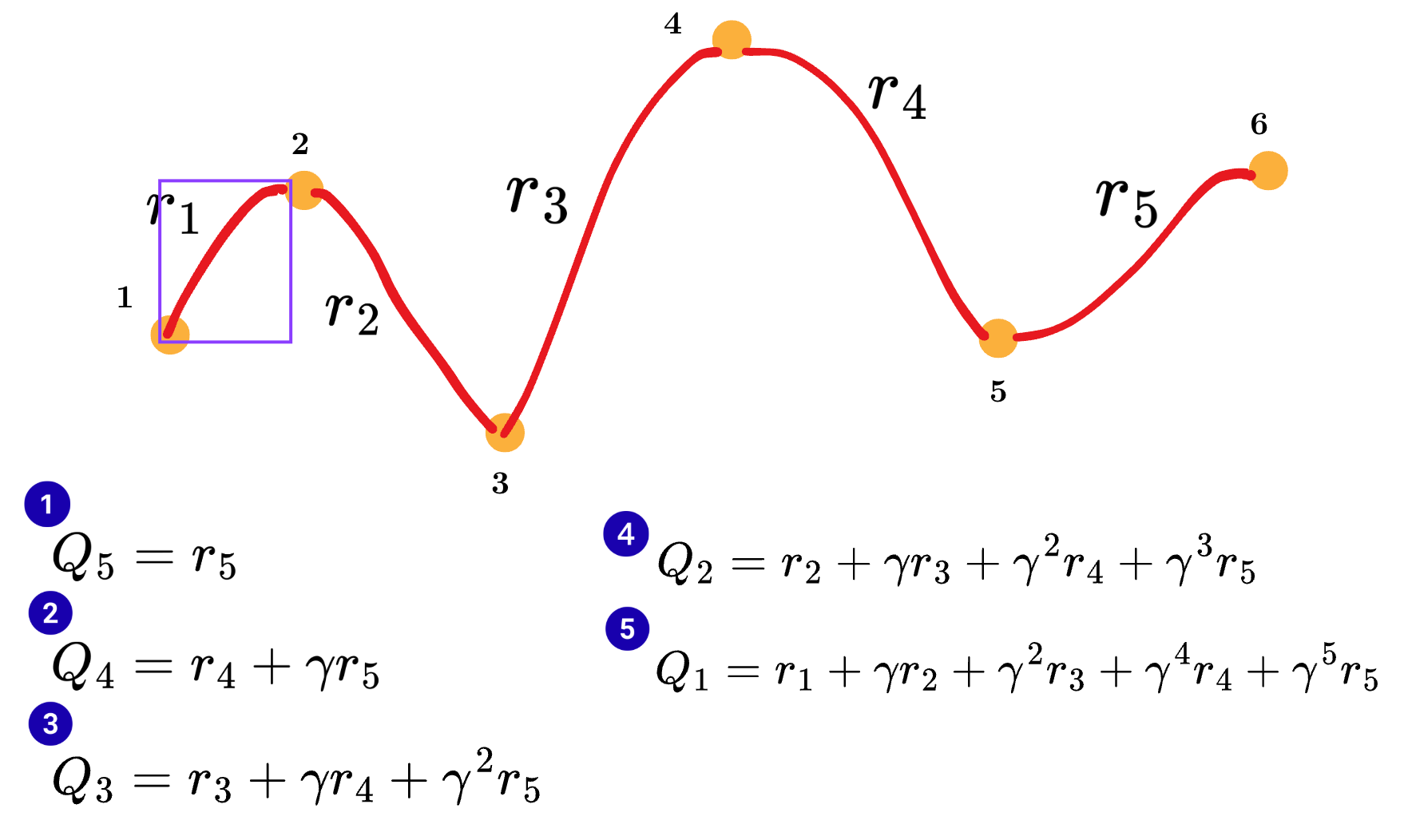
First, we calculate the return from the last state and then use that information to calculate the return of the previous state, and so on, until we reach the first state of the episode.

Remember that we will be using this Q-value in the policy update rule where it will be multiplied with the grad log probabilities.

Step 3: Collect states, actions and rewards

This is done using the following piece of code:

# --- Action Selection ---
            # Convert state to a tensor and add a batch dimension
            state_t = torch.as_tensor(state, dtype=torch.float32)
            
            # Get action probabilities from the network
            logits_t = net(state_t)
            probs_t = F.softmax(logits_t, dim=0)
            
            # Sample an action from the probability distribution
            # .item() extracts the value from the tensor
            action = torch.multinomial(probs_t, num_samples=1).item()

            # --- Environment Step ---
            next_state, reward, done, truncated, _ = env.step(action)

            # --- Store Experience ---
            # We store the state, action, and reward for the currentstep
            batch_states.append(state)
            batch_actions.append(action)
            episode_rewards.append(reward)

From the above code, we can see that the actions are sampled from the probability distribution which our policy neural network generates.

This action is then passed to the “env.step( )” function to collect the next_state and the reward.

Step 4: Loss Calculation and Optimization

In this step, we calculate the gradient of the performance measure and perform the gradient ascent rule to update our model parameters.

Here is how we write the code for this step:

# --- Loss Calculation and Optimization ---
        optimizer.zero_grad()
        
        logits_t = net(states_t)
        log_prob_t = F.log_softmax(logits_t, dim=1)
        
        # Get the log probabilities for the actions that were taken
        log_prob_actions_t = log_prob_t[range(len(batch_states)), actions_t]
        
        # Calculate the policy loss: - (log_prob * Q-value)
        # We want to maximize (log_prob * Q-value), which is:
        # minimizing its negative.
        loss_t = -(qvals_t * log_prob_actions_t).sum()

        loss_t.backward()
        optimizer.step()

In the above step, you can see that we are calculating the log probabilities for the actions, multiplying them by the Q-value, and then summing it up for all the states in the episode. This is exactly what the REINFORCE algorithm says.

This can be shown in the following figure:

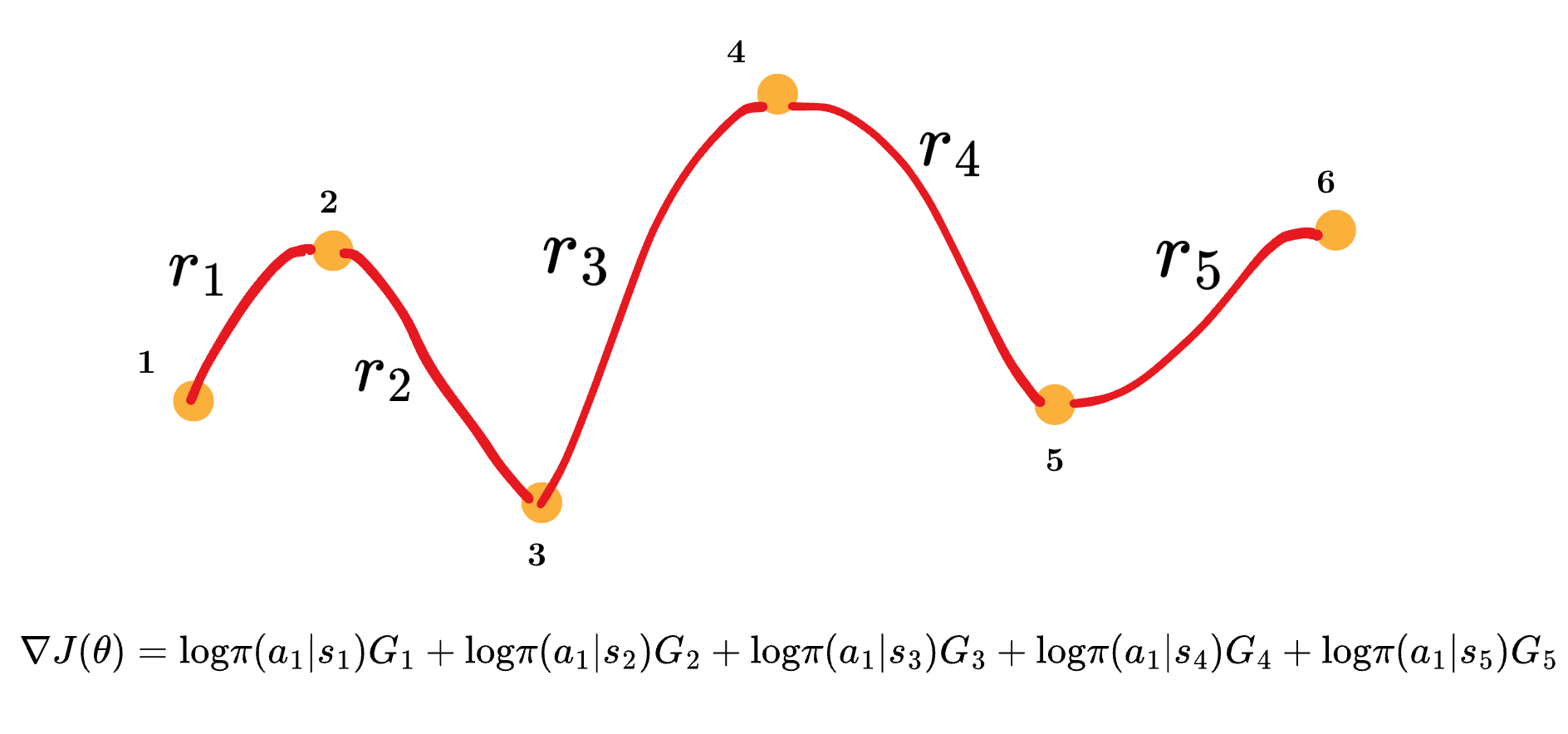
We multiply this gradient with a negative sign, because, for the Python library, we need a loss which we can minimize, not maximize.

Now we have all the pieces of the puzzle ready, let us see how the rewards change with time.

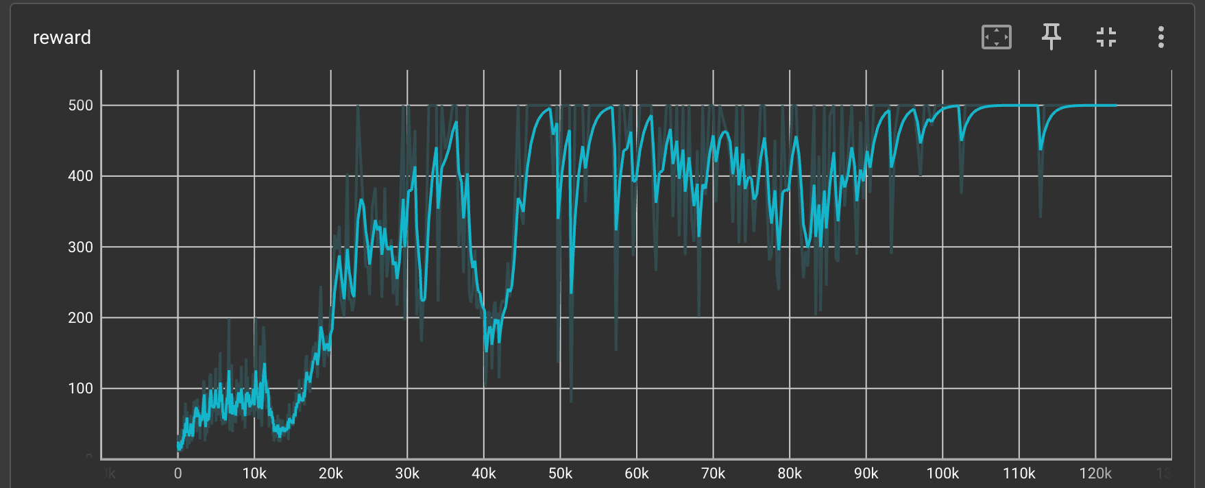
We can clearly see that the reward increases with time and reaches a value of 500, which is excellent.

We also plot the variance of the Q-values to check whether the variance is indeed an issue with the REINFORCE method.

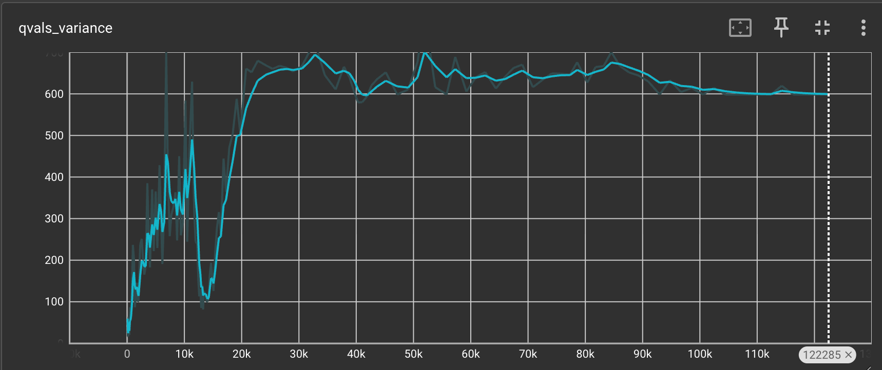
The variance values seem to be quite large and they exceed 600 at one point.

Now let us run the code by using REINFORCE with Baseline method.

We are only going to do one small change in the code where we are going to subtract the Q-values with a baseline.

We are going to use a baseline which is the mean of all the Q-values that have been encountered in the episode so far. This will make sure that any unnecessarily high or low values do not get unnecessary weightage when calculating the gradients.

def calc_qvals(rewards: tt.List[float]) -> tt.List[float]:
    """
    Calculates discounted rewards for an episode and applies a baseline.
    The baseline is the mean of the discounted rewards for the episode.
    Subtracting it helps to reduce variance.
    Args:
        rewards: A list of rewards obtained during one episode.
    Returns:
        A list of baseline-adjusted discounted total rewards (advantages).
    """
    res = []
    sum_r = 0.0
    for r in reversed(rewards):
        sum_r *= GAMMA
        sum_r += r
        res.append(sum_r)
    
    # Reverse the list to match the order of states and actions
    res = list(reversed(res))
    
    # Calculate the mean of the discounted rewards (the baseline)
    mean_q = np.mean(res)
    
    # Subtract the baseline from each discounted reward
    return [q - mean_q for q in res]

Now let us compare the rewards for both the methods:

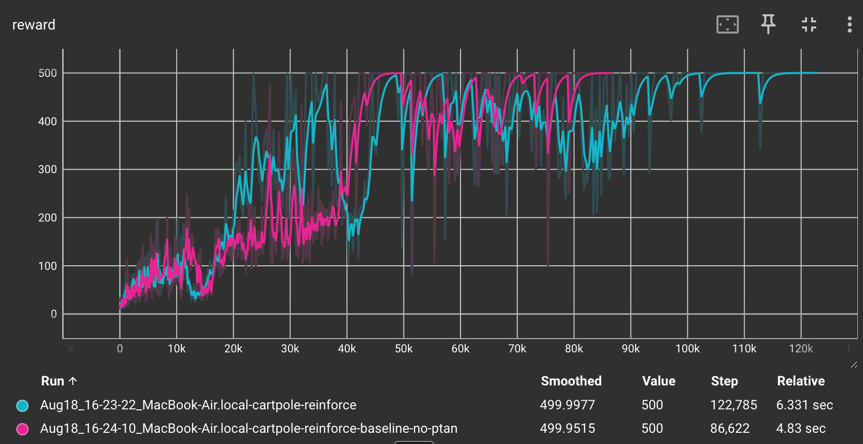
We can see that the REINFORCE with Baseline method (shown in pink) reaches to a reward of 500 much faster, in 86,000 steps as opposed to 120,000 steps required for the simple REINFORCE method.

Let us check the variance of the Q-values.

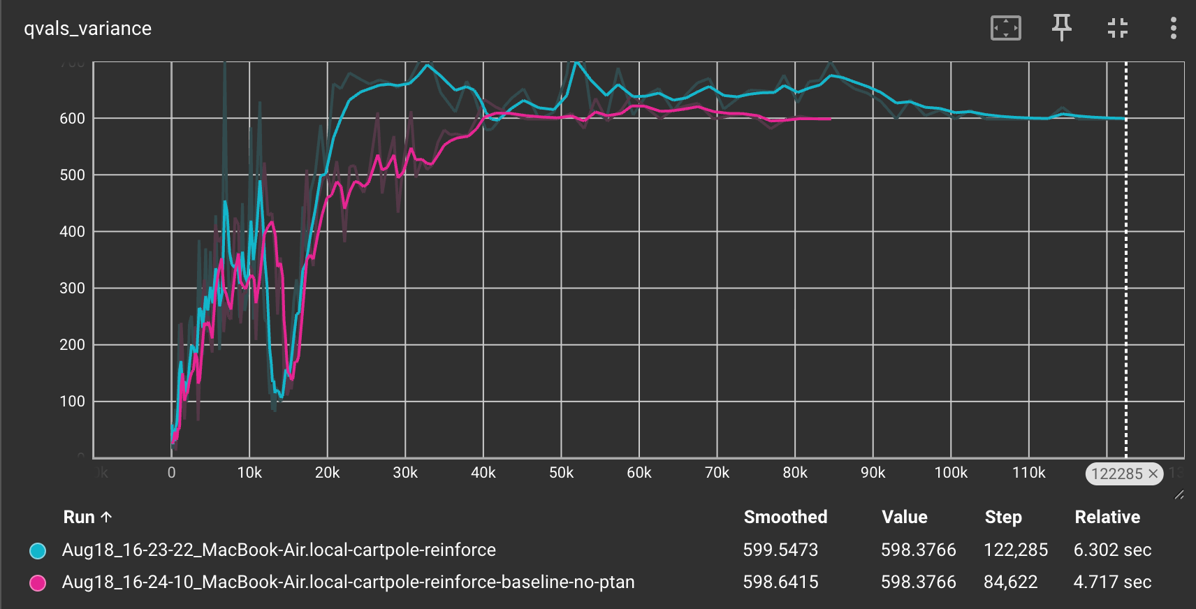
The Q-value variance is significantly less for the REINFORCE with Baseline method compared to the simple REINFORCE method.

This clearly tells us that introducing a baseline not only reduces the variance but also allows for faster convergence.

Refer to this GitHub repo for reproducing the code: https://github.com/RajatDandekar/Hands-on-RL-Bootcamp-Vizuara