
Regularization : What? Why? and How? (Part -1)
Regularization from a visual mathematical lens


What would have been your approach towards regularization if you were the person who actually came up with it? Are you unable to connect different concepts which we generally see while learning about Regularization? Maybe due to the isolative way we learn about this or the lack of general tools you need to crack this up. If you are a discoverer by heart, and love to read, glide through this article/story and see your dots connect.

Every story has a monologue, then why not here? So, let’s start,
Since the advent of problem solving/optimization, specifically Deep learning as a problem solving field, a lot of time went into finding optimal and quicker way to solve problems. But most of research works which tried solving a problem using Deep neural nets as a single function failed to work at scale; mostly because they were trying to do something called as unconstrained optimization or solving without bounds (don’t worry we will talk about this term later). Only after inclusion of constraints/regularization and few other techniques quick advancements began to happen. But why were they failing in general and how did regularization fixed some issues?

Lets understand this by first understanding overfitting.
The dataset which we assume to be significant enough to train our model, is a discretized subset of true continuous population distribution.
Thus we can’t be sure that; even if we fit a perfect model on this, we will be perfectly fitting over the true distribution, and our main task was to approximate true distribution! This gives way to situation called overfitting. As the Bias (How close is your trained model to the best-possible model; on average) is very low which is defined by

Where f’(x) is your trained model and f(x) is the perfect/best-possible model(best model which could be trained on given dataset which we consider part of true distribution; but significant enough to represent true distribution), on the given chunk of dataset, not the entire population.
and the Variance (How much your per sample prediction is varying as compared to mean of your model predictions) is high (sensitive model) which is defined by,

So, what are implications of this high variance and low bias?
It means your model is complex. In general ML sense, complexity could be referred to two situations, first, if there are too many learnable parameters, second if the parameters are having high degree of freedom to grow (that is their coefficients are unbounded), both of these conditions makes model/approximator very sensitive to the observed samples.
To be more clear; let’s try to understand it again with a simple analogy,
If there are large number of parameters, each parameter could be mapped corresponding to each input then we would end up learning a highly complex function. It is similar to eating soup with a very large spoon, will it do the task? Yes, is it worth it? No. On the other hand, if there is large accumulation of weight, this will make model very sensitive to small changes in input, and thus model will be highly unstable, again not a desired situation.
So, if we reduce model complexity somehow, then we will overcome overfitting? Yes, Occam’s razor also symbolizes the same thing, a simpler model is always better, and this is where regularization steps in.
Regularization helps by penalizing any sort of complexity, maybe complexity due to large number of parameters or large accumulation of weight.
We can perform regularization by doing either; or both of the below mentioned things,
1. constraining number of parameters
Sparsity plays a very major role in this. A general idea to understand this could be, that if network is sparse, number of learnable parameters will be low, thus complexity would reduce, preventing model from overfitting.
2. constraining size of parameter values
Putting penalty over the parameter values, This is generally done by adding a penalty term in cost function, which has an regularizing effect. i.e. if the parameter values/weights get too large our cost function accounts for a large loss. We will see this more clearly in later section.
Both of the above mentioned points could be used in conjunction with each other as well. Like, a penalty term that accounts for larger weights as well as sparsity as in case of L1 regularization. We have an entire section on L1 and L2, so, bear with me.
We saw some new terms in last few paragraphs, like cost function, penalty term and constrained/unconstrained optimization. Lets see how they fit into the big picture.
In first two paragraphs, I started by saying that issue is that we were trying to solve an unconstrained problem then I suddenly jumped to complexity and overfitting, seems fishy, right? Yes, a bit, so let’s connect them together now,

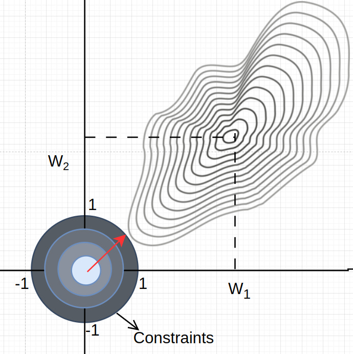
In the diagram above, the spirally thing at top-right is our distribution that we want to approximate. On axis we have our parameters, so one thing is for sure, if model has to fit the distribution it needs to move along w1 and w2 axis. (Fitting of a distribution means approximating statistic of a distribution like mean and standard deviation or more abstractly as moment estimation).
This is the moment of truth, w1 and w2 could grow arbitrary large to fit the distribution, which would make our model complex and would cause overfitting, which meant that we were trying to solve an unconstrained problem, or simply this was an unconstrained optimization.
But, now one could ask why not just normalize data onto fixed domain and then try to fit it. Few things that we have to keep in mind while thinking on this framework is
We are working on subset of true population (the best we can do is sample-level normalization) which anyways won’t standardize or normalize your true distribution, it will still be shifted and spread out (becomes harder for complex domain), hence, again your model has to be complex (large w1 and w2) to fit the shape, eventually the actual information lies in the direction not in magnitude; hence we want to restrict the magnitude aspect of things here).
For me, regularization serves as surface or problem simplification or smoothening. Imagine you are asked what is the shape of your phone, rectangle-ish? square-ish? trapezium-ish? all of these -ish assumptions are simpler yet similar approximation of actual complex surface with complication borders/boundaries. But, this is a good approximation, as you can answer a lot of interesting questions like length, area, volume, etc. without ever knowing the exact criterions. This simpler assumption could be more precise (both in terms of magnitude and point sparsity); hence fitting data more perfectly (imagine fitting a complex contour with two parameters, the best they can draw is a circle, what if we go to a higher yet limited number of parameters). Now, this was scenario in 3d, just imagine what would happen in much higher dimensions/higher degree of freedom, with some mathematical guarantees these methods shine much brighter than we estimate.

Few interesting points to notice from above diagram, given sufficient freedom we can approximate the data, also the shape of assumption defines a lot of things. Due to few interesting properties the optima of actual shape and current shape coincide (which we will skip here, but you can read about level sets).
Let’s look it in this was as well, given you want to write a function y = f(x), where x is [1 ,1], and expected y is presumably 4. Parameters of f are w1 and w2. In how many ways can we combine them to get expected y, using a linear system of equations.

w1 and w2 could be anything literally, in the range of (-∞, ∞), which will satisfy the equation.
4 = 4*1 + 0*1
4 = 100*1 + (-96*1)
4 = (-500*1) + 504*1

We also want to put more focus to the parameters/features with more importance w.r.t. to our data. So, our best bet could be to not allow weights to get larger than a certain point or simply to constrain the weight values for better control and gradient computations.
As we know that larger weights means high complexity and thus leads to overfitting in most cases. And the solution which we saw above was to put some restriction/constraints over the parameter values. Thus, I think the link should be clear between unconstrained optimization and overfitting. But how do we actually play with this optimization thing and what exactly is it? Let’s discuss that in the next section.
What is Optimization?
In general machine learning sense, it is solving an objective function to perform maximum or minimum evaluation. In reality, optimization is lot more profound in usage.
 Meme Meme Generator")
Then we have two terms which we hear often with “optimization” as suffix. Convex/non-convex optimization and linear/non-linear optimization. For linear and nonlinear optimizations, the name is quite evident of our task at hand. It is literally solving a system of equations, which might be linear or non-linear. But as far as convex and non-convex go, they are a bit different, there could be entire blog on these two guys, thus we will gently pick the things we require and then move on.
Points we need to know:
1. If Hessian/second derivative/Jacobian of gradients of cost function is all positive then the function is convex, if all negative then concave, and if mix of both, then the function is non-convex.

2. For intuition purpose, hessian defines curvature of function, imagine there is a U-shaped curve, like y = x², if you draw any line connecting any two points on the curve, all the points in between will lie below the curve. Thus curvature is below the straight line. Now imagine drawing many lines f(a)-f(b) and if it hold true for all, then it should be convex. But if it fails at some location then it is non-convex. Homework for you, this connects why there is more risk of encountering saddle points while training our models as compared to local minima.
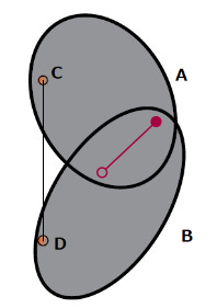
3. We know what convex and non-convex functions are, let’s talk operations over them, what if we add two convex functions? what do we get? The answer is the intersection of two convex functions (f1+f2) will always give a convex function, but a convex and non-convex together will give a non-convex one. But two non-convex might end up giving a convex surface (not very useful here, but has an intricate implication in loss and weight space). This is the reason why we generally see things similar to combinations of multiple L1 or L2 terms, as both are convex and thus could be optimized.
4. But why only convex optimization? For a long time it was speculated that considering a problem as hard is about linearity versus non-linearity, but later it was concluded that it’s mostly about convexity and non-convexity. Actually, convex problems are the only ones for which we have some deterministic method for solution; that is by using KKT conditions, thus we want to restrict ourselves in the domain on ONLY CONVEX (for more info you can explore about complexity theory and completeness). Maybe, in future we come up with a way to deterministically solve non-convex problems as well, but for now let’s relish on what we have, and be curious about what we don’t.
Great! We know now what convex optimization is and why is it important. We have our tool stack ready to discover Regularization ourselves. Congrats on that first of all. Give yourself a pat on shoulder for this. Let’s start the process to discover Regularization.
We mentioned that we wanted to put some restriction/constraints over our parameters value. But how do we do that? ask yourself, we want a function which could give a high penalty every time w1 or w2 gets larger than our threshold (k).

P(w) is ∞ if y > k; otherwise it is 0 (k is the threshold, could be assumed 0 here).
isn’t this what we wanted? now let’s add up this term to our actual objective function, which generally is a MSE or MAE (which are also convex as per our requirement for optimization).

But P(W) given current discrete setup behaves like a standard step function, as there is sudden penalty/loss as soon as we step out of our threshold range. This would result in unhealthy gradient flow.

Imagine if threshold is 1 and our f(W) is 1.0001, still we would see a huge loss, which is not good, to make things a bit smoother we make a linear dependency between P(W) and a new term lambda (λ).

Interestingly enough, even after using our linear dependence λ*P(W), the actual objective remains same, as below equation on maxima would give step function again (when lambda goes to ∞).
Our new equation after this became,

Does it remind you of something? yes, it’s the familiar equation you generally see while learning about Regularization. This lambda which we talked about is your so called “regularization parameter or mathematically as lagrange multiplier”, which is said to balance objective term and penalty term, but does lot more than that as we saw above.
You saw that we can add a penalty term to our objective, but what if we add multiple of them? A general equation should look like,

This entire equation together is called as lagrangian. So, you can define lagrangian as boxing of your main objective function with all the penalty terms/regularization terms.
Now these penalty terms could be anything, could be l2 norm (results into L2 regularization) or L1 norm(results into L1 regularization) or combination of both(yes, you are right, elastic net). Wasn’t it intuitive?
Now, let’s get a bit technical, we wanted to minimize our main objective function which was MSE right? And we want to give large penalty when we cross threshold using penalty term. Thus we can see the equation as,

From Game theory perspective, You can think of this as a min-max game, optimizing MSE results in larger W, on the other hand optimization of P results in smaller W. The only sweet spot to optimize (minimize) both of these functions together is at boundary/threshold of P.
From Machine learning perspective, you can understand it like this, the weights value would account for larger penalty as they grow larger, as soon as they grow enough to touch our distribution, they would stop growing, because any value above that, though would reduce MSE but would account for very heavy penalty as well. Thus, this boundary act as sweet spot for optimization.
Now, we are almost done, we know that just adding this regularization term to our main objective function would result into a new objective function whose optimization would prevent us from overfitting (because of min-max game we discussed just now).
We have multiple options for defining P(W), it could be L1/L2/ L1 + L2 or anything, but it should be convex.

We now have the equation of regularization setup completely, just some insights on choice of P is left. As we are accounting for metrics of weights thus most obvious choice is the usage of something which we refer as Norm (which we will discuss in next part).
With this we conclude our part-1, and learnt about optimization and its conjunction with complexity, we also hovered through convex vs non-convex optimization, we also saw a general mathematical yet easy to understand perspective for formulating a combined objective function and hence finally reaching our target : The regularization equation. In the next article we will pick up from here and understand about our choice of P(W) from a machine learning perspective.
Thank you for being curious enough to read through this entire article, and yes, give a pat on your shoulder again, you learnt something new today. I will catch up with a new article sometime in future. Till then, keep exploring and learning. Bye.