
1-bit LLMs : The final frontier for Large Language model optimization
Ultra-low precision models are redefining efficiency, not just for inference but for training too. Imagine building and using powerful LLMs even on low-end GPUs. The era of being GPU-poor is ending.

Table of content
Introduction
Why 1-Bit (Ternary) Models Are the Final Frontier?
Why 1-bit (ternary) is the "final resolution wall"?
Why reaching here is a breakthrough?
Problems Associated with Ultra-Low Precision
Error Accumulation at Lower Precision
Presence of Non-Differentiable Blocks
Less Resolution Space → Reduced Degree of Freedom → Activation Collapse
Now, Why 1-bit is way Worse?
Solutions to Tackle Ultra-Low Precision Challenges
How 8-bit and 4-bit Training Managed These Challenges?
FP4 Training: Recent Advancements
BitNet
What Problems BitNet Aims to Solve and Major Contribution?
BitNet: Design and Deep Intuition
Energy Advantage Table
Comparisons and Results
Potential Issues with BitNet
The Ideal Case: What Would a Perfect Low-Bit LLM Look Like?
BitNet v2: Native 4-bit Activations with Hadamard Transformation for 1-bit LLMs
Methodology
Example setup
Experiments & Summary of Design, Metrics, and Results
A quick deep-dive into Post-ROPE quantization and ROPE fusion
Final thoughts
Conclusion
Introduction
In recent years, the growth of Large AI models has been nothing short of exponential. From vision transformers to large language models, we have seen models balloon in size crossing hundreds of billions of parameters. With this explosion comes an undeniable challenge: resource constraints. Memory bottlenecks, energy consumption, and training time are reaching unsustainable levels, especially as the industry moves toward training trillion-parameter scale models.
This is where low-precision training steps in as a transformative technology. By reducing the number of bits used to represent model weights, activations, and gradients, we can significantly cut down both memory footprint and computational cost which is often by factors of 2x, 4x, or even more. However, making this shift without sacrificing accuracy or stability is a non-trivial task.
In our previous blog

we explored these concepts in depth. We started by laying down the fundamentals around precision:
Why precision matters in machine learning
What exactly "model precision" means, and how it relates to concepts like floating-point representation (mantissa, exponent, sign bits)
How precision compares to something familiar like image resolution
Why bit reduction mainly targets the mantissa and how it helps both in speed and efficiency
Challenges that arise due to lower precision, such as error accumulation and gradient underflow
We then discussed how quantization is generally performed, and the practical techniques engineers use across different stages:
During training: through Mixed Precision Training
Post-training: through Post-Training Quantization (PTQ)
During fine-tuning: through methods like QLoRA
During inference: using ultra-low precision formats like INT4 and beyond
Finally, we dived deep into the specific challenges faced in 4-bit training, like the need for proper quantization of activations, handling dequantization through Differentiable Gradient Estimators (DGEs), and the general methodology for achieving forward and backward passes in low precision. We rounded it off by discussing experimental results and reflecting on key thoughts.
In this article, we take the next step.
We will explore the ambitious world of 1-bit training; pushing the limits of quantization even further.
We will build this exploration around two important works:
BitNet: The first practical framework showing how to train neural networks with binary or 2-bit weights.
BitNetV2: An improvement over BitNet, solving many of its shortcomings, and scaling 2-bit training to even larger, more complex models.
Our goal is not just to understand what these papers achieved, but to deeply internalize how they made it possible despite the formidable barriers standing in the way.
Why 1-Bit (Ternary) Models Are the Final Frontier?
In the journey toward ultra-efficient training, we first moved from 32-bit floating point (FP32) to 16-bit (bfloat16/fp16), then to 8-bit (INT8), then even down to 4-bit (NF4, FP4, INT4). Each step squeezed models tighter, making them faster, lighter, and cheaper to train.
However, once you start imagining 1-bit or ternary models where each weight can only be -1, 0, or +1, you are truly at the endgame of precision compression.
Why 1-bit (ternary) is the "final resolution wall"?

An intuitive way to understand this is by thinking about image resolution or grids on a map.
With high-bit (like 32-bit), you are operating on an ultra high-resolution map, hence tiny details, curvy rivers, intricate borders can all be precisely drawn.
At 8-bit or 4-bit, the resolution drops as the map starts getting a bit blocky, but most important features are still visible.
At 2-bit (or ternary 1-bit), you are working with a super low-resolution map; almost like big square tiles.
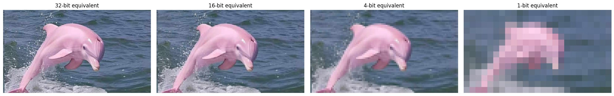
And when you push to 1-bit, you have only 3 choices for every point:
Raise (+1)
Lower (-1)
Stay flat (0)
There are no finer details left. No subtle hills or valleys. Either a sharp bump up, a sharp dip down, or flat ground. Imagine trying to sketch a mountain range with only those three instructions. The nuance and grace of the shape almost disappear.
Similarly, when training LLMs, the model loses expressive freedom to capture fine patterns.
This can also be thought over in terms of movement freedom, imagine a character moving inside a space.
At 3-bit precision, it's like moving freely inside a cube, you can go up, down, left, right, forward, and backward (full 3D motion).
At 2-bit precision, you're restricted to a square plane, now you can only move up, down, left, or right, hence losing one degree of freedom (no vertical movement).
Finally, at 1-bit (ternary) precision, you're confined to a single line; you can only move left, right, or stay in place hence drastically limiting your choices.
This shrinking of movement mirrors how reducing precision cuts the model’s degrees of freedom:
the lower the precision, the less flexibility the model has to "navigate" the complex landscape of optimization. At 1-bit, you're operating almost on rails while forcing the model to learn with minimal expressive capacity, making training extremely delicate.
Thus, 1-bit or ternary models represent the absolute limit:
Go lower, and it’s just a flat surface.
No structure, no learning.
Why reaching here is a breakthrough?
If we can make 1-bit (ternary) models work, then training massive LLMs becomes insanely efficient:
Memory bandwidth becomes a non-issue.
Models can be deployed on much cheaper hardware.
Energy consumption drops dramatically.
Scaling to trillion-parameter models becomes much more feasible.
This is why BitNet is an important milestone. It attempts to reshape the Transformer itself to operate robustly even when parameters are aggressively quantized to {-1, 0, +1}, though going to exactly 0 is hard (we will see in the quantization step)
Problems Associated with Ultra-Low Precision
As we aggressively reduce numerical precision; from 16-bit to 8-bit, then 4-bit and now towards 2-bit, we don't just get faster computation. We also start breaking some of the fundamental assumptions that make deep learning work in the first place.
Let’s go through the three big issues that arise:
1. Error Accumulation at Lower Precision
In standard (fp32) training:
Tiny gradient updates are accumulated accurately over time.
Even small changes help the model descend the loss landscape precisely.
In ultra-low precision:
Tiny updates get rounded off or completely lost during quantization.
Gradients that are smaller than the quantization step vanish entirely.
Example:
If your quantization step size is 0.5, and you compute a gradient of 0.1,
then in quantized math, 0.1 → 0.
Thus, information is irreversibly lost, leading to inaccurate or stalled learning.
2. Presence of Non-Differentiable Blocks
Many quantization functions (like rounding, clamping, sign functions) are non-differentiable by nature.
During backpropagation:
The chain rule needs gradients to flow smoothly.
Non-differentiable points introduce sharp discontinuities.
Approximating them using tricks like STE (Straight Through Estimator) only partially solves the issue.
At lower precision, the entire model becomes sprinkled with more non-differentiable components, making gradient-based optimization fragile and noisy.
3. Less Resolution Space → Reduced Degree of Freedom → Activation Collapse
Neural networks thrive on rich, diverse activations:
Different neurons fire differently to encode different features.
When you reduce precision:
The range of values neurons can represent shrinks drastically.
Many neurons end up producing the same output values, no matter what the input is.
This is called Activation Collapse:
The model stops being able to differentiate between inputs.
Learning grinds to a halt because everything starts looking the same internally.
Now, Why 1-bit is way Worse?
Everything mentioned above becomes exponentially more severe when we go to 1 bits.
Let's revisit the three problems under 1-bit specifically:
1. Error Accumulation Becomes Catastrophic
With only 2 values to represent all real numbers, even medium-sized gradients get completely rounded off.
Fine-tuning, subtle corrections during training which are essential for convergence become almost impossible.
Example:
Imagine needing to adjust a weight from 0.0 to 0.2 to improve accuracy.
In 2-bit, there's no “0.2” you either stay at 0.0 or jump directly to 1.
This mismatch destabilizes training.
2. Non-Differentiable Zones Everywhere
In 2-bit:
The "quantization function" behaves like a hard, staircase function.
The derivative is zero almost everywhere and undefined at the step points.
Thus, using standard gradient descent techniques becomes almost meaningless without extra tricks (approximations, smoothing, etc.).
3. Activation Collapse is Almost Guaranteed
Using the map/grid analogy again:
At 2-bit, each neuron can only output 4 distinct values.
It's like labeling every country on Earth as just "A", "B", "C", or "D", the subtle differences between regions (or features) are completely lost.
Thus, the model's expressivity collapses:
Different input patterns produce identical activations.
The model can't differentiate cats from dogs anymore as everything looks like a vague "animal" category.
Quick Note:
Many of these issues were discussed in detail in my previous article where we covered:
Why error accumulation occurs naturally when reducing mantissa bits,
How mixed-precision training (forward pass in low precision + full-precision master weights) tries to compensate,
Why activation scaling is essential to prevent neuron dead zones.
(Refer to sections like:"But, why does error accumulation happen?", "How Engineers Handle Precision to Scale LLMs", "Ideal situation, problems associated and proposed solution for 4-bit training".)
Thus, the problems are not new, but at 1-bit, they hit with such brute force that traditional remedies start failing, hence, prompting the need for fundamentally new ideas like BitNet.
Solutions to Tackle Ultra-Low Precision Challenges
As we discussed earlier, ultra-low precision introduces serious challenges:
Gradients disappearing due to rounding errors,
Instability during backpropagation,
And a collapse of neural expressivity.
However, the community has not sat idle over the years, several clever engineering techniques have been developed to mitigate these issues, especially in the 8-bit and 4-bit training regimes.
Let’s first revisit how these problems were traditionally handled, and then show why these methods start to fail when we move to 1-bit training.
How 8-bit and 4-bit Training Managed These Challenges?
A. Mixed-Precision Training
Instead of using low-precision everywhere,
Forward Pass:
Compute activations and loss in low-precision (e.g., bfloat16, fp8) for speed.
Backward Pass (Update):
Keep a master copy of the weights in fp32 (full precision).
Update these master weights with accurate small gradients.
This ensures:
You enjoy the speed-up of low-precision,
Without sacrificing the subtle adjustments needed during learning.
B. Loss and Activation Scaling
Small gradients can vanish in low-precision math. To prevent this:
Scale up activations and loss during computation,
Then appropriately scale them down during updates.
This tricks the system into preserving tiny but crucial gradients.
C. Regualarizing range of activations
As discussed in paper : An Empirical Study of μP Learning Rate Transfer, the authors maintain the activations such that the their range (which is actually in full FP16/32 precision) doesn’t leak beyond FP8 which could then be simply converted to FP8 while doing forward propagation.
FP4 Training: Recent Advancements
In the FP4 training framework for LLMs (discussed in my earlier article), two major innovations helped stabilize 4-bit training:
Differentiable Gradient Estimator (DGEs):
Instead of using hard rounding during backpropagation, use a soft differentiable approximation,
Thus gradients can flow more reliably.
Outlier Clamping and Compensation (OCC):
Special handling of rare big values (outliers) that could distort the distribution after quantization.
Together, these innovations made 4-bit training not only possible but effective. But, as we saw in the sections above as soon as you jump to 1-bit, the surrounding problems worsens by order of magnitudes hence rendering the solutions more or less useless.
BitNet
In this work, a scalable and stable 1-bit Transformer architecture designed for large language models is introduced. Specifically, authors introduce BitLinear as a drop-in replacement of the nn.Linear layer in order to train 1-bit weights from scratch. Experimental results on language modeling show that BitNet achieves competitive performance while substantially reducing memory footprint and energy consumption, compared to state-of-the-art 8-bit quantization methods and FP16 Transformer baselines. Furthermore, BitNet exhibits a scaling law akin to full-precision Transformers, suggesting its potential for effective scaling to even larger language models while maintaining efficiency and performance benefits.
What Problems BitNet Aims to Solve and Major Contribution?
As deep learning models, especially LLMs, grow into hundreds of billions of parameters, reducing the compute and memory footprint becomes absolutely critical. While previous methods have explored 4-bit or 8-bit quantization successfully, the biggest computational bottleneck which is matrix multiplications is still largely done at relatively high precision.
BitNet sets out to radically change this by asking:
Can we push the matrix multiplication itself the heaviest operation inside Transformers down to 1-bit precision, and still train a competitive model?
BitNet introduces several innovations that allow them to preserve model quality while binarizing the majority of computation:
BitLinear layers: special binary matrix multiplications that use +1 and -1 weights instead of full-precision numbers. This serves as drop-in replacement of conventional
nn.Linearlayer in the transformers.High-precision critical components: BitNet selectively retains high precision (8-bit or full precision) for parts that matter less to compute but are critical for stability, like:
Residual connections and Layer Normalization, which add little computational cost.
QKV transformations in attention, which are relatively lightweight compared to the larger projections.
Input/output embeddings, where precision is vital because sampling from language distributions needs high accuracy.
Maintaining training stability through careful variance control (LayerNorm before quantization) and smart scaling (β and γ factors).
Simply put, BitNet identifies the real heavy parts of the Transformer and compresses only those, while protecting the fragile but essential parts with higher precision.
BitNet: Design and Deep Intuition
BitNet keeps the overall Transformer structure (stacked self-attention and feedforward blocks), but replaces all expensive dense layers (matmuls) with "BitLinear" operations.
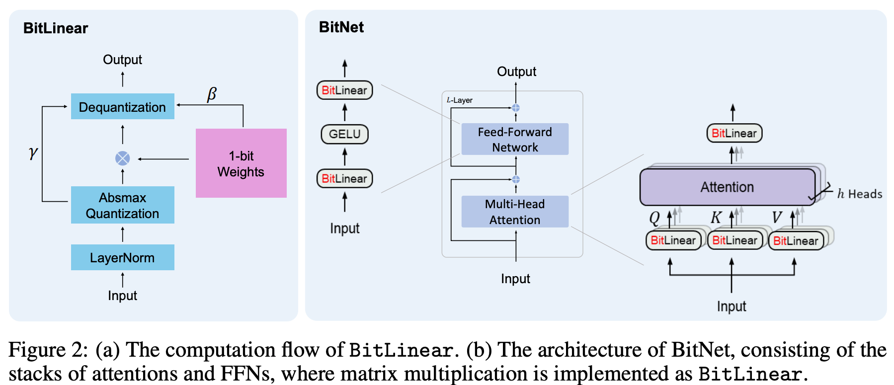
Here's how it works:
1. Binarizing Weights
In standard matrix multiplication, weights are continuous values like 0.245, -0.837, etc.
BitNet simplifies this drastically:
Each weight is mapped to either +1 or -1 using a sign function after zero-mean centralization (to balance the number of +1 and -1).
Mathematically:
Subtract the mean α from all weights so that they center around zero.
Apply the Sign function:
+1 if value > 0
-1 if value ≤ 0
The process works like this:
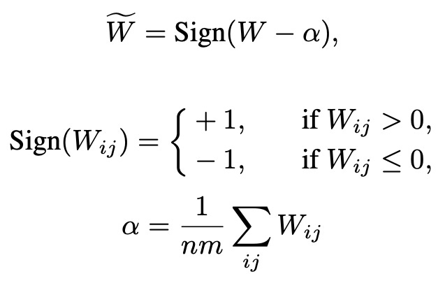
where:
Wf is the original weight matrix (full precision).
α is the mean value of all weights.
Sign(⋅) is the signum function:
+1 if positive
-1 if zero or negative.
Binarization is like performing hard selection instead of softly blending multiple directions like full-precision weights do, you either fully activate a feature or completely reject it. It's no longer a matter of "how much" you move in a direction (magnitude), but simply "yes/no", do you move along that basis vector or not. In other words, it's like navigating a space with only the compass directions (north, south, east, west) rather than fine-grained degrees.
2. Scaling with β
Because binarization loses magnitude information, BitNet introduces a scaling factor β, proportional to the average absolute value of the original weights, to minimize the l2 difference between real and binarized matrices.
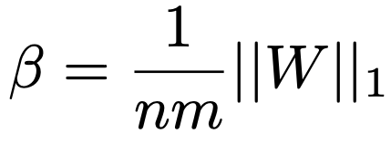
This scaling ensures that although weights are now binary, their "effective strength" is still somewhat preserved during the matrix multiplication. β acts like a "volume knob" that tries to restore how strong or weak the original weights were. Without β, every binarized weight would be treated equally strong, destroying important relative differences.
3. Quantizing Activations
Activations are not binarized (doing so would be catastrophic). Instead:
Activations are scaled into a fixed range using absmax quantization.
The largest absolute value (γ) in the tensor is used to rescale everything into a manageable range; e.g., for 8-bit, between -127 and 127. This is becuase that activations can have wild dynamic ranges, hence, f you just naively scale, huge outliers could ruin quantization.
A tiny ε is used during clipping to avoid overflow.
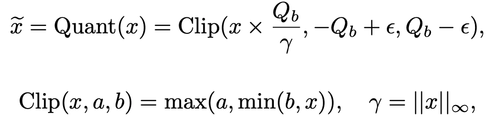
Where:
Qb=2^b−1 : maximum value for bbb-bit quantization (for 8-bit, Qb=128Q_b = 128Qb=128).
γ=∥x∥∞ : largest absolute value in x.
ϵ is a tiny offset to avoid overflow during clipping.
Clip(x,a,b)=max(a,min(b,x)) is simply activation clipping based on maximum activation value
Before non-linear operations (like ReLU), activations are shifted so that they become non-negative (by subtracting the minimum value) and quantized again.
4. Matrix Multiplication at 1-bit
Now, the BitLinear matrix multiplication happens between:
1-bit weights (+1 or -1)
8-bit quantized activations
Since both operands are highly compressed, the multiplication becomes extremely lightweight, hence, much faster and more memory-efficient than traditional float16 or float32 matmuls.
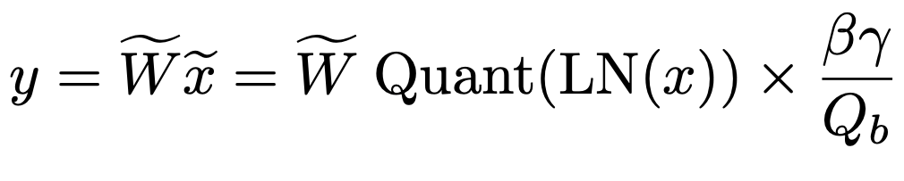
After the multiplication, results are rescaled back (using β and γ) to restore their approximate magnitude.
5. Maintaining Training Stability
A big problem with quantization is variance mismatch. Full-precision models initialize weights such that the output variance is around 1 (using Kaiming or Xavier initialization), which helps gradients flow smoothly.
BitNet solves this by applying a LayerNorm (SubLN) before activation quantization.
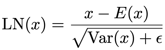
This standardizes activations: mean 0, variance 1. After this, activations are nicely centered and scaled, making quantization much more stable and predictable. Ensuring that activations have unit variance even after aggressive compression helps in maintaining similar dynamic ranges as in full-precision models, thus preventing instability or vanishing/exploding gradients.
combining everything, the final equation looks like,
6. Model Parallelism with Group Quantization and Normalization (important)
One major hurdle in scaling large language models is model parallelism, dividing large matrix operations across multiple devices like GPUs. However, quantized models like BitNet introduce new difficulties in parallel computation.
The Problem
BitNet needs to compute global statistics like α (mean of weights), β (mean absolute value), γ (max of activations), η (min of activations) as well as mean and variance for LayerNorm (SubLN).
But traditional model parallelism assumes the tensor partitions are independent. So if one GPU only holds a slice of a tensor, it cannot compute global stats without a communication-heavy all-reduce operation. This becomes a bottleneck, especially as models go deeper.
The Solution: Group Quantization & Group Normalization
To fix this, BitNet proposes a simple idea: Group the tensors, and compute all quantization and normalization stats within each group independently.
Group Quantization for Weights
Given a weight matrix W, we divide it into G groups along the partition dimension. Each group is of size (n*m)/G. Then for each group g, we calculate:
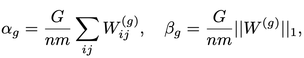
here W(g) denotes the g-th group of the weight matrix.
Because of this, each GPU can compute αg and βg locally, eliminating the need for global synchronization.
Group Quantization for Activations
Similarly, for input activation matrix x∈(n×m), we group along rows and compute:
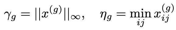
Again, local stats only, hence, no all-reduce required.
Group Normalization
Even LayerNorm (which normally depends on the full tensor’s mean and variance) can be made parallel by applying Group Normalization:
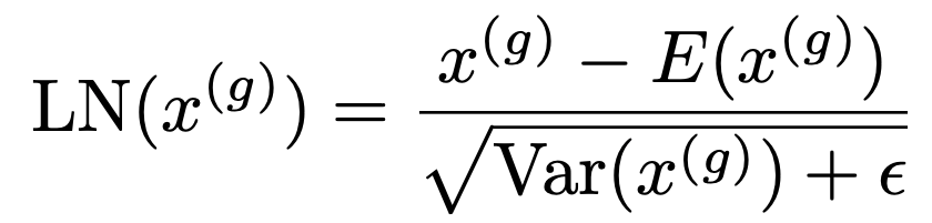
This ensures each partition (GPU) does its own normalization, independently.
7. Model Training Strategies
Even with a smart forward pass, training a quantized model like BitNet isn’t trivial. Here's how the authors made it work:
Straight-Through Estimator (STE)
Operations like Sign() (Eq. 2) and Clip() (Eq. 5) are non-differentiable. Hence, backpropagation can't flow through them directly.
So BitNet uses the Straight-Through Estimator, which just pretends these functions are identity during backward pass. You can fins more information about this in our previous article.
In other words:
Forward: Do the binarization/quantization
Backward: Let gradients flow as if no quantization happened
Mixed-Precision Training
Although weights and activations are quantized for forward/backward:
The latent weights (underlying real weights) are stored in high precision (e.g., FP32).
Optimizer states (momentum, etc.) are also in high precision.
Why? Because tiny updates to a 32-bit float might have no effect after binarization. So you need full-precision storage to accumulate updates to ensures stable training.
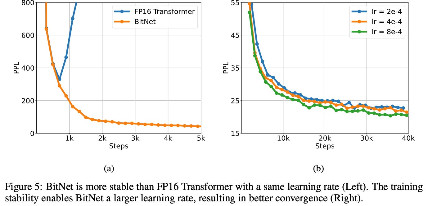
Large Learning Rate
Here’s an interesting observation from the paper:
“A small gradient update to the latent weight often doesn’t flip its 1-bit binarized version.”
This makes early training slow as the model can’t “move” because binarized weights don’t change. So the solution? Crank up the learning rate.
This encourages:
Larger weight movements that flip bits.
Faster early convergence.
Remarkably, BitNet tolerates higher learning rates better than FP16 Transformers, which often diverge with aggressive learning (You can also connect this to the flat surface/manifold analogy, as the surface is extremely smooth now, we can take really long strides without much disturbances).
Energy Advantage Table
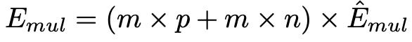
BitNet’s hardware efficiency is real. A simpler way to measue this is by calculating the energy from the formula mentioned below
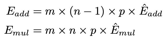
For BitNet, the energy consumption of the matrix multiplication is dominated by the addition operations, as the weights are 1-bit. The multiplication operations are only applied to scale the output with the scalars β and γ Qb , so the energy consumption for multiplication can be computed as:
Here’s a snapshot from the paper’s energy comparison table (using 512 tokens):
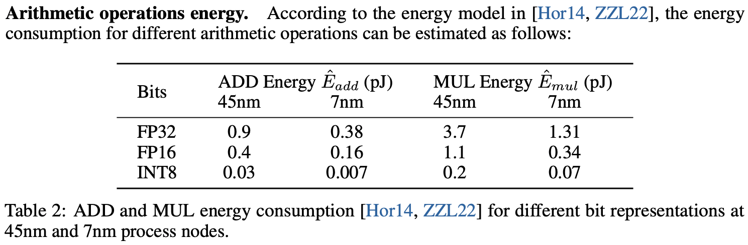
BitNet provides significant energy savings, especially for the multiplication operations, which are the major component of the matrix multiplication energy consumption.
Comparisons and Results
Sure, here’s a more concise and insightful summary:
Setup : BitNet models (125M–30B) are trained on English corpora using SentencePiece (16K vocab) and compared with FP16 Transformers under identical conditions.
Inference-Optimal Scaling Law
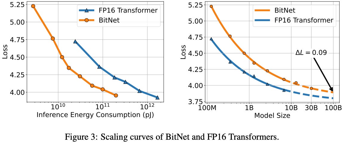
BitNet matches FP16 Transformers in power-law loss scaling, but achieves better performance per unit of inference energy, highlighting its superior efficiency.
Downstream Tasks
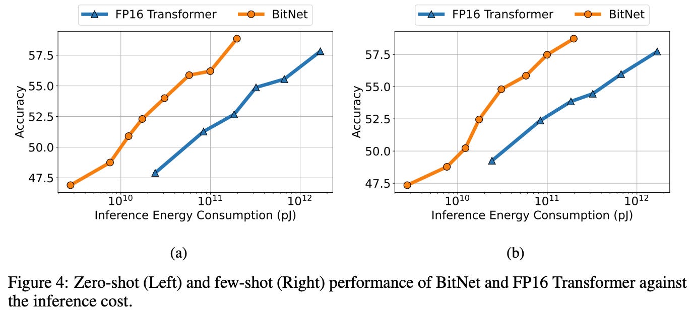
BitNet scales more effectively in zero-shot and few-shot performance across tasks like HellaSwag and Winograd, outperforming FP16 models as size increases.
Stability Test

BitNet shows greater training stability, tolerating higher learning rates and converging better than FP16 models, aiding faster and more robust optimization (probably because the gradients are quite smoothed; hence the loss function is way less noisy, thus even with larger steps you are more or less in usable plane).
Comparison with Post-Training Quantization
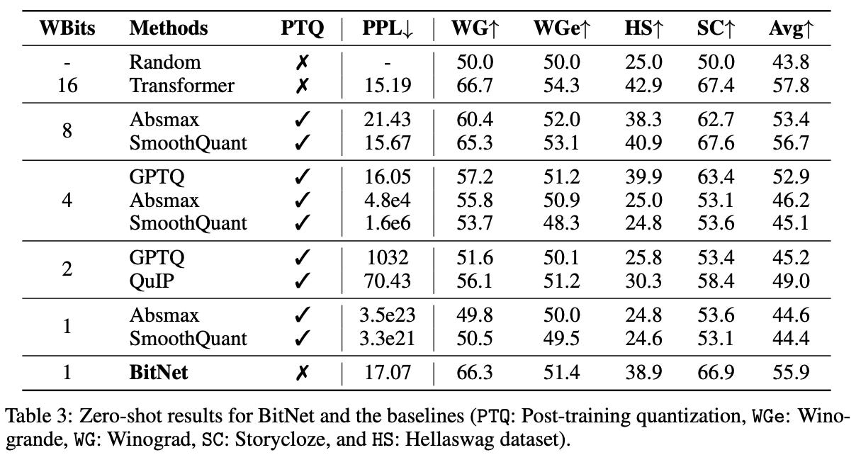
BitNet (W1A8 or weight with 1-bit precision and activation with 8-bit precision) outperforms state-of-the-art post-training quantization methods at lower bit levels, showing that quantization-aware training is more effective than retrofitting precision reduction.


BitNet consistently achieves higher accuracy and lower perplexity than alternative low-bit methods, validating its design across both zero-shot and few-shot settings.
Potential Issues with BitNet
Despite its efficiency gains, BitNet has several key limitations that cap its scalability and hardware utilization:
8-bit Activations as Bottleneck
While weights are 1-bit, activations remain 8-bit, limiting gains on hardware optimized for 4-bit computation and increasing memory and latency overhead.Hardware under-utilization
BitNet can’t fully exploit next-gen GPUs (example, GB200) with native 4-bit support, since activations prevent fully low-bit matmul kernels.Outliers in Intermediate Activations
Attention and FFN layers often produce spiky, non-Gaussian outputs, making aggressive quantization error-prone without further processing.Model Parallelism Challenges
Global parameters (α, β, γ, η) break tensor independence, requiring costly synchronization unless grouped (Group Quantization), which adds complexity.Training Overheads
Despite 1-bit weights, training relies on full-precision latent weights and gradients. Small updates often get masked in binarization, requiring high learning rates and careful tuning.
The Ideal Case: What Would a Perfect Low-Bit LLM Look Like?
An ideal low-bit LLM would not just reduce memory costs via 1-bit weights, it would holistically embrace low-precision across the full computation pipeline, without compromising performance or scalability. Here's what such a setup would look like:
Truly End-to-End Low Precision
Instead of just binarizing weights, the model would operate with sub-4-bit activations throughout, especially in the attention and feedforward block, hence, unlocking the full efficiency of next-gen accelerators like GB200.Distribution-Aware Quantization
The model would reshape or regularize outlier-heavy intermediate activations (common in FFN/attention blocks) to enable aggressive quantization, without loss in expressivity. Techniques like Hadamard transformations or dynamic quantization ranges can help in achieving this.Communication-Efficient Model Parallelism
Ideal model parallelism would eliminate the need for costly all-reduce operations by computing parameters like α, β, γ, η locally within tensor groups (via group quantization and normalization), ensuring scalability across nodes without synchronization penalties.Optimization Stability Without Precision Trade-Offs
The training loop would maintain high precision only where absolutely necessary (e.g., latent weights, gradients), and apply robust strategies like Differentiable Gradient estimators (DGE) and adaptive learning rates to mitigate gradient masking.Hardware-Aware Design
Architecturally, the model would align with the parallelism, memory layout, and throughput characteristics of modern AI hardware, enabling batched inference with dense low-bit kernels that favor speed and energy efficiency.
Some of these challenges had been discussed and potentially tackled in recent paper named : BitNet v2: Native 4-bit Activations with Hadamard Transformation for 1-bit LLMs, lets dive directly into understanding the delta that BitNet v2 talks about.
BitNet v2: Native 4-bit Activations with Hadamard Transformation for 1-bit LLMs
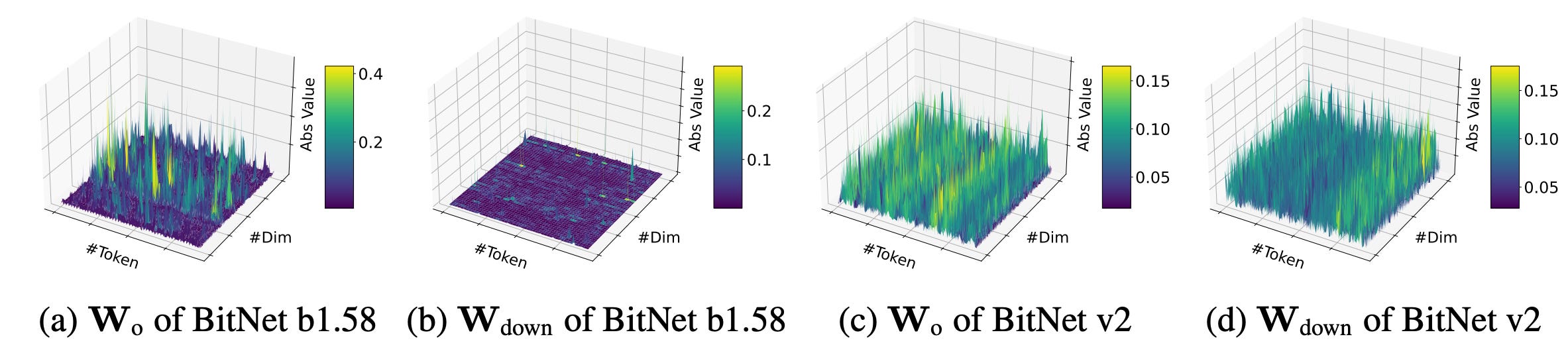
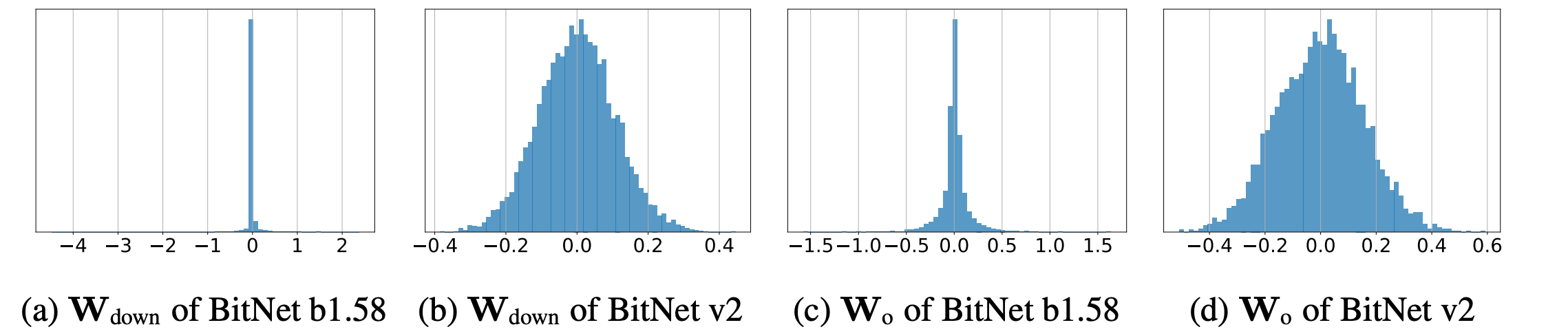
Just to put things in more perspective, BitNet v2 claims few major changes:
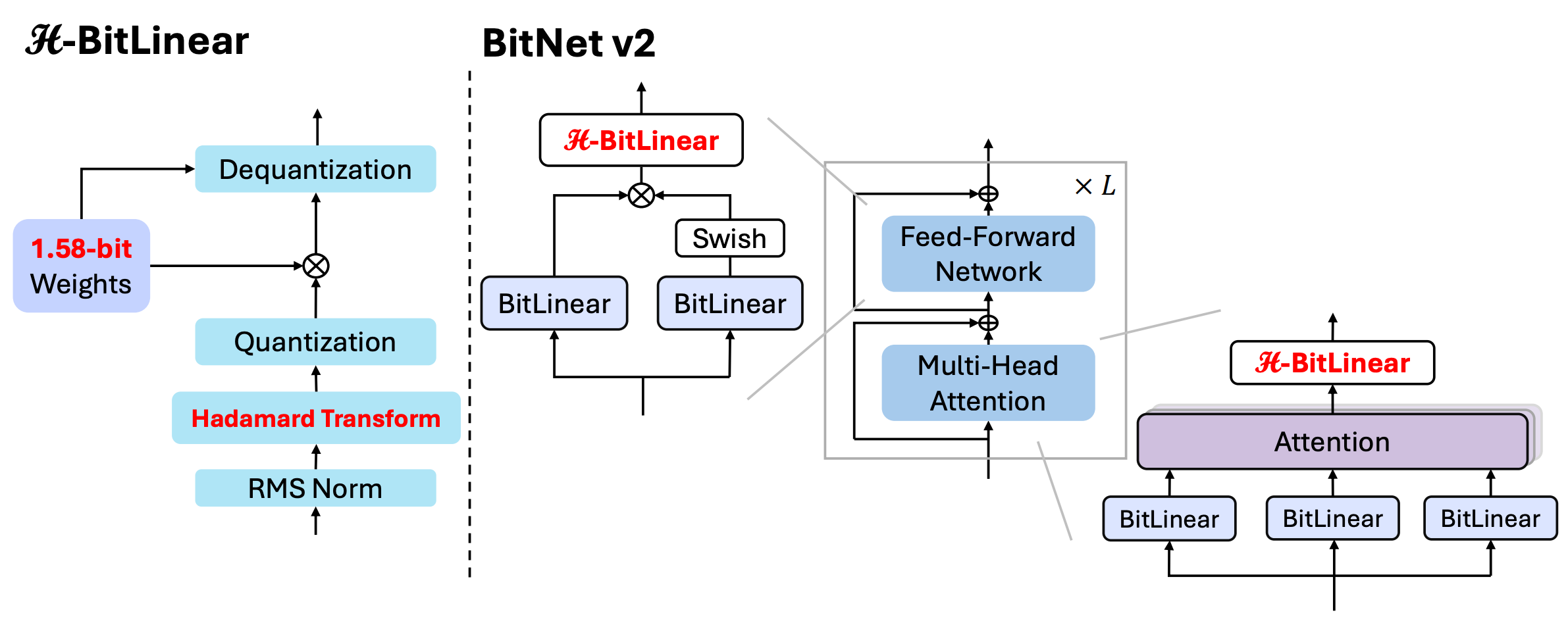
Introduced H-BitLinear, replacing standard
WoandWdownlayers to better handle activation outliers.Applied a Hadamard transformation before activation quantization, reshaping sharp distributions into Gaussian-like forms for smoother low-bit quantization.
Enabled native INT4 activations (except input/output embeddings), using per-token absmax and absmean for quantization.
Leveraged the orthogonality of the Hadamard matrix to enable efficient backward propagation through the transform.
Maintained latent full-precision weights and used STE with mixed-precision training for optimization stability.
Lets go through each component and discuss in detail
METHODOLOGY
1. Weight Quantization (Ternary Quantization)
Weights are quantized to 3 values:
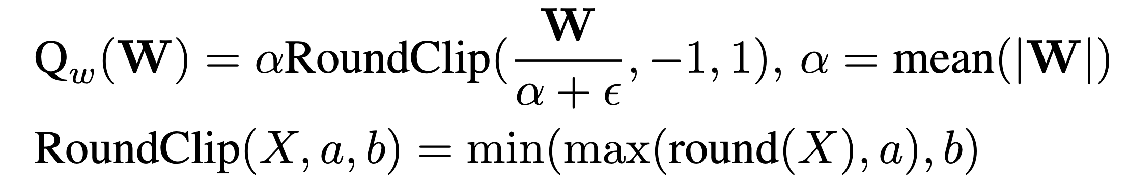
The use of ternary quantization here is deliberate. It aligns with BitNet's core philosophy of extreme compression without training collapse.
Why mean-based scaling? Because it provides a robust and stable scaling factor even in presence of outliers (unlike max, which gets skewed). This makes ternarization resilient and expressive enough, while still being cheap to store and compute.
And using RoundClip keeps the values safely bounded in {−1,0,1}, which is critical for bit-efficient matrix multiplications in hardware. You can also think of it as baked in hard feature selector.
2. Hadamard Transformation Before Activation Quantization
Before we quantize the activations (especially the intermediate ones from Wo and Wdown), we apply:
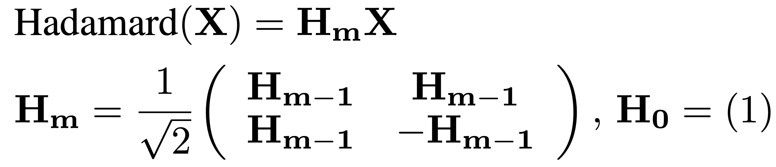
where Hm=recursive orthogonal matrix
But why do we even need this step?
Because raw intermediate activations are messy, they're often spiky, contain outlier-heavy channels, and aren’t friendly to low-bit quantization. That’s where Hadamard comes in. Lets give this a bit more space to understand it better.
Is Hadamard like channel-level averaging?
On first look it seems like a sort of mean shifting or averaging. Though it is similar in spirit:
Both mix information across channels.
Both aim to smooth out irregular distributions.
But it’s not “just averaging”:
Averaging kills structure.
Hadamard does structured mixing with +1s and −1s, hence it doesn’t just add-everything-up. Its more like spreading the information across all the features such that energy of the system before and after remains same. Whereas mean though spreads out value but it behaves as a smoothening operation, hence, reducing the quality of features.
This is why:
It preserves total information (via orthogonality).
It balances the signal across channels, so no single dimension explodes.
Yet, it’s super lightweight in terms of computation, it is just O(nlogn) with the Fast Hadamard Transform.
Think of Hadamard like this:
A carefully scrambled remix of the data.
It's like "spreading out the signal energy" without flattening the music.
Instead of having one channel with 5.0 and others with 0.0, you get a balanced remix like:

→ Now quantization doesn't choke on that 5.0; the information is well-distributed and has higher degree of freedom.
3. Activation Quantization
Once the activation has been transformed and normalized, they apply bit-specific quantization:
INT8
It is done through below mentioned formulation. Here we can see that they shift the signal and then clip between (-128, 127), while scaling by γ which simply is max of signal. Hence, we can define the process as normalization followed by clipping.

Why max-based scaling? Because INT8 has more dynamic range, and max ensures that we fully utilize all 8 bits. But it’s riskier for lower-bitwidth.
INT4:
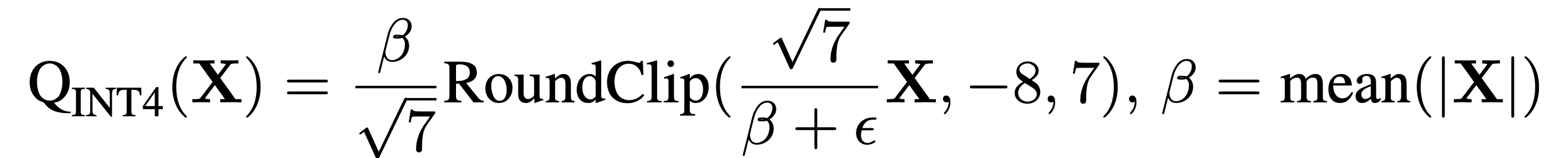
Notice the switch to mean-based scaling for INT4 (this is subtle but smart).
At lower bitwidth, max is volatile which means a single spike can ruin the whole batch.
Mean is more stable and gives better bit allocation across the full activation range.
Also, why the sqrt(7) factor? Remember the range for INT4 (2^4) hence (-8 to 7)? It’s a normalization trick to map mean values into the available quantization levels, minimizing clipping.
4. Final Linear Output
So the full transformed, quantized matmul looks like:

That’s the core machinery of H-BitLinear.
It’s a delicate sandwich: Normalize → Hadamard-mix → Quantize → Multiply by ternary weights.
Each step exists to tame distribution and squeeze performance out of limited bits.
5. Training & Backpropagation
They use STE (Straight-Through Estimator) for quantization which is a standard trick to enable gradient flow through non-differentiable steps, I have discussed about this in detail in my previous blog.
For Hadamard, they lean on a beautiful property:
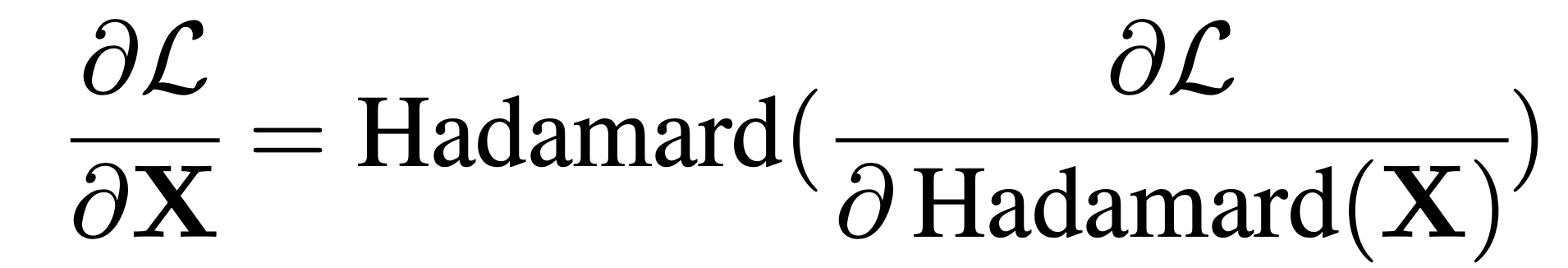
This works because the Hadamard matrix is orthogonal, so its inverse is just itself (Linear algebra 101). Also during training, they maintain latent full-precision weights for updates, hence keeping training smooth and stable. They only quantize for the forward/inference path with all the above discussed tricks.
Now, we know the theory part, why not lets understand the forward pass with a real example
Example Setup
Lets assume that we have a toy 4D activation vector (must be power of 2 for Hadamard):
Clearly, there's a huge outlier in the last channel, this would cause problems in low-bit quantization.
Case 1: Direct INT4 Quantization (No Hadamard)
We use mean-based scaling for INT4:
Mean of abs values:
\(\beta = \text{mean}(|X|) = \frac{0.02 + 0 + 0 + 5.00}{4} = 1.255\)Quantize:
\(Q_{\text{INT4}}(X_i) = \beta \cdot \frac{1}{\sqrt{7}} \cdot \text{RoundClip}\left( \frac{\sqrt{7}}{\beta} X_i \right)\)
Compute scaling factor:
Now quantize each value:

Result:
This results in severe compression of the outlier, everything else becomes 0, hence, massive information loss.
Case 2: With Hadamard Transformation Before Quantization
Step 1: Apply Hadamard (4x4 version)
Then:
Step 2: Compute mean:
Scale:
Now if we Quantize each:
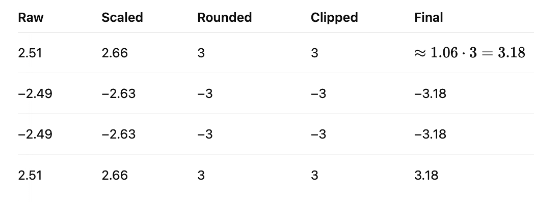
Result:
And as we can see, this gives a Balanced representation, no spike gets cut off, information is spread evenly.
In summary, we can clearly conclude that
Without Hadamard:
All channels except one collapse to zero.
The outlier gets clipped hard.
With Hadamard:
All channels contribute.
Information is balanced across bits.
Quantization becomes more efficient and fair.
Experiments & Summary of Design, Metrics, and Results
Baseline Setup
Compared against:
BitNet b1.58: INT8 activations.
BitNet a4.8: Fine-tuned from b1.58, with 4-bit inputs and top-K sparsified intermediate states.
SpinQuant and QuaRot: Post-training quantization baselines using 4-bit activations and GPTQ-like techniques.
BitNet v2 Training Setup
All models use 1.58-bit ternary weights.
Two-stage training:
Stage 1: Train with 8-bit activations on 95B tokens.
Stage 2: Continue-train with 4-bit activations on 5B tokens.
Post-RoPE quantization for QKV projections.
Absmax quantization: No calibration data needed.
Kept [BOS] KV cache at 8-bit for stability in long contexts.
Evaluation Metrics
Perplexity (PPL) on C4 validation set.
Zero-shot accuracy on 6 language understanding benchmarks:
ARC-Easy (ARCe), ARC-Challenge (ARCc)
HellaSwag (HS), PIQA (PQ)
Winogrande (WGe), LAMBADA (LBA)
Average Accuracy reported across these tasks.
Results/Outcomes
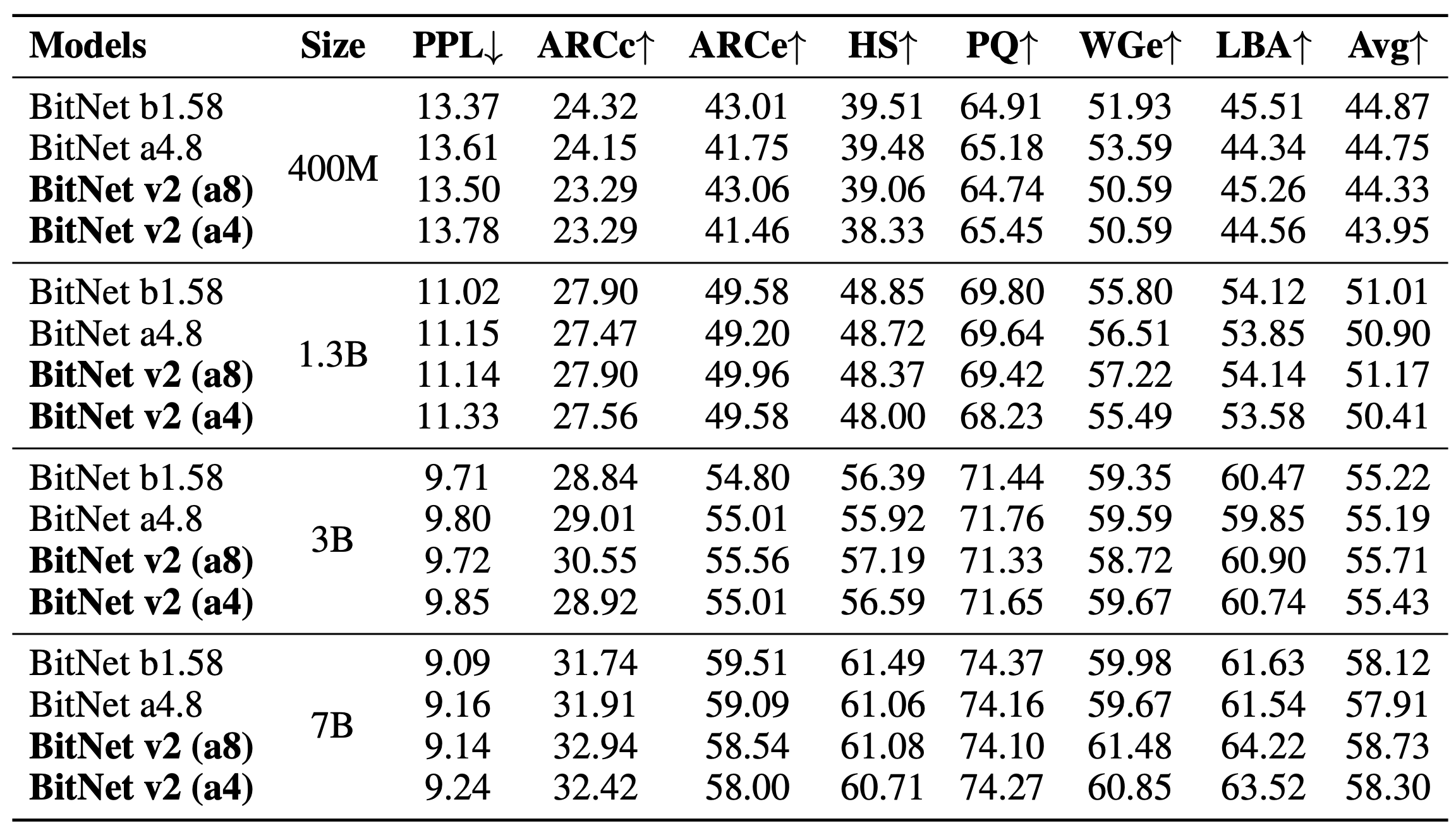
1. BitNet v2 vs b1.58 and a4.8
BitNet v2 (a8) outperforms b1.58 on downstream accuracy across model sizes:
+0.16% (1.3B), +0.49% (3B), +0.61% (7B)
BitNet v2 (a4) matches or beats BitNet a4.8 in accuracy while being fully 4-bit (no hybrid).
Perplexity remains comparable or better despite lower bit activations.
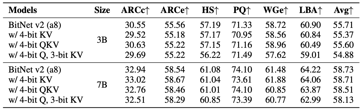
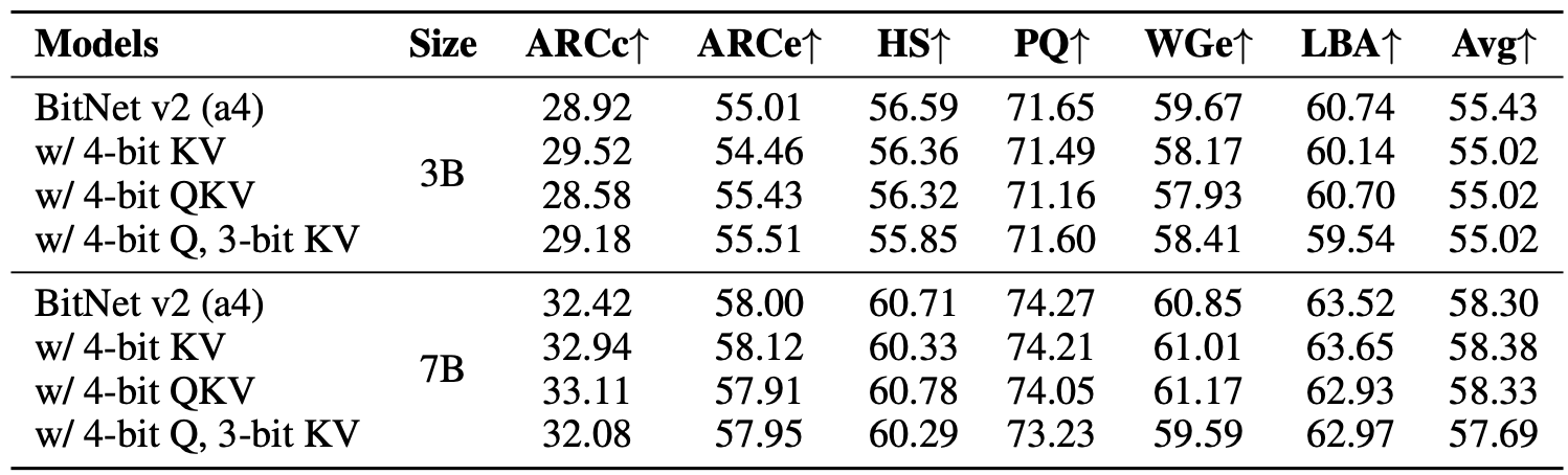
2. QKV Bit-Width Sweeps
3-bit KV cache maintains accuracy close to 8-bit KV.
e.g., 3B model with 4-bit Q, 3-bit KV hits ~54.88% avg accuracy, vs 55.71% for full 8-bit.
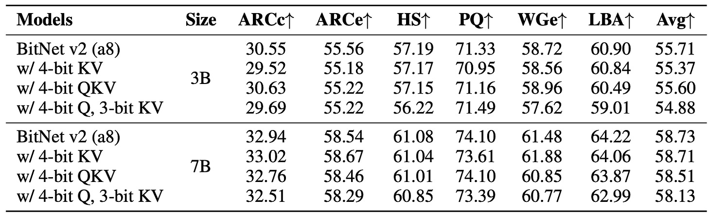
The zero-shot accuracy of BitNet v2 with 8-bit activations and QKV states varying bit-widths on the end tasks.
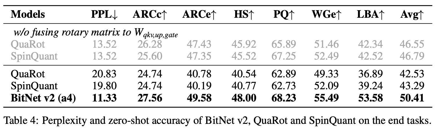
3. BitNet v2 (a4) vs Post-Training Quantization
On 1.3B models:
BitNet v2 achieves PPL: 11.33, Avg Accuracy: 50.41%
QuaRot and SpinQuant achieve PPL > 19, Avg Accuracy: ~42–43%
Thus, BitNet v2 is 7–8% more accurate and much more efficient.

The zero-shot accuracy of BitNet v2 with 4-bit activations and QKV states varying bit-widths on the end tasks.
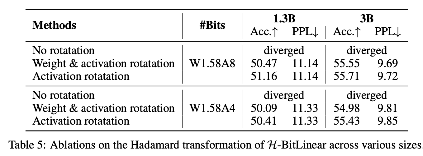
4. Hadamard Ablation
Without Hadamard: model diverges.
With Hadamard on activations only: stable and high-performing.
Full Hadamard on both weights & activations gives faster convergence but similar end performance.

when the authors remove rotary fusion (i.e., don’t pre-rotate weights), the performance improves significantly
5. Rotary Fusion Ablation
Fusion of RoPE into weights (W·RoPE) degrades performance for ternary models.
Better to apply RoPE separately (Q(W) · RoPE).
SpinQuant’s PPL drops from 19.80 → 13.52 with this fix, but still trails BitNet v2.
A quick deep-dive into Post-ROPE quantization and ROPE fusion
Most of the points in above section are clear and straightforward, but, I think two of them need special attention.
Post-RoPE quantization
Fusion of RoPE into weights (W·RoPE)
Lets dive a bit into them for better understanding
Q1 : Why Post-RoPE quantization?
Lets see the setup first, Assume that we have a set of vectors xi∈Rd each of which contain some meaningful high-dimensional representations (e.g., token embeddings). These vectors are unique, or at least distinct in subtle but important ways. Now, lets say that there's a rotation matrix RRR, like the one used in RoPE, that applies a position-dependent transformation to these vectors. Finally, Then there's quantization, which squashes vectors into a coarse grid, hence limiting their ability to express fine detail.
Case 1: Quantize First, Then Rotate
If you quantize first, you take your high-resolution vector x and reduce its values to coarse levels. For example: a float vector like [0.57,1.03,−0.45][0.57, 1.03, -0.45][0.57,1.03,−0.45] becomes [0.5,1.0,−0.5][0.5, 1.0, -0.5][0.5,1.0,−0.5]
Now, several distinct vectors collapse into the same or very similar quantized versions. Their geometry is blurred. When you now apply the rotation matrix R, you're rotating these already flattened vectors.
So even after rotation, the output vectors don’t spread out much. They cluster, because their inputs were similar to begin with. It's like rotating a bunch of identical sticks, they rotate, but they all look alike. This results in loss of information happens before you had the chance to enrich or differentiate.
Henceforth, vectors lack diversity → poor expressivity → weak performance.
You can imagine this as blurring a canvas and then painting/sketching on the low resolution space.
Case 2: Rotate First, Then Quantize
Lets Start with the same rich, floating-point vector x. The we apply rotation matrix as R.x, now the vector encodes positional/geometric variation in addition to its semantic meaning. Even similar vectors now diverge slightly based on position, phase, or frequency modulation introduced by RoPE.
Now quantize the result. Yes, there’s still precision loss; but this happens after you've enriched the representation. So, even though the quantized vectors are coarse, they reflect more distinctive directions. This results in Quantization compressing a space that was already populated with diverse, position-aware vectors, hence, you retain more useful signal.
Opposite of previous example, You can imagine this as painting/sketching on a high resolution space and then blurring it, now you have more degree of freedom.
Hence, to conclude,When quantization happens after rotation, it preserves more distinct structure, because rotation spreads out the data beforehand. When it happens before, the structure is already flattened, so rotation just moves around bland, uniform vectors
This understood, lets move to the next question.
Q2 : Why Fusion of RoPE into weights (W·RoPE) is bad?
Before even answering this, What is "Rotary Fusion"? In some quantized models (like SpinQuant or QuaRot), they fuse the Rotary Positional Encoding (RoPE) matrix into the projection weight matrices.
That is, instead of doing:
Q = (X @ W_q) # projection Q_rotated = RoPE(Q) # apply rotary afterwardThey fuse RoPE into weights and do:
W_q_rot = (W_q x RoPE) # merging / pre-rotating
Q = X @ W_q_rot # pre-rotated weights
here @ is (matrix multiplication) and × is (element-wise multiplication or sometimes symbolic fusion)
This is called fusion of RoPE into W_q, the rotary matrix is pre-multiplied into the weights. This saves runtime ops as we are saving one multiplication step, but has side effects in low-bit models. Now we know the basics, lets try to understand why its problematic for low-precison models.
Ternary or quantized weights (like BitNet’s 1.58-bit weights) are very sensitive to small changes. When you fuse RoPE into W_q, you’re forcing those projection weights to encode not just the normal projection task; but also positional encoding logic.
In a quantized regime, that:
Adds unnecessary complexity to a fixed, lossy matrix (the ternary W_q)
Causes loss of expressiveness during learning
Leads to worse generalization (especially in attention-heavy tasks)
In contrast, BitNet v2 avoids this fusion, doing RoPE as a separate, online operation after projection, hence, keeping each layer’s job clean and focused. Here W_q just projects and RoPE just rotates after which we simply apply quantization.
Final Thoughts
BitNet v2’s carefully engineered activation transformations (Hadamard + quant), post-RoPE quantization, and efficient training schedule deliver state-of-the-art performance at low-bit precision while outperforming baselines both in perplexity and downstream accuracy, while enabling full INT4 inference.
Interestingly, through these modifications they were able to beat BitNet a4.8 and BitNet b1.58 (previous iterations) across multiple benchmarks.
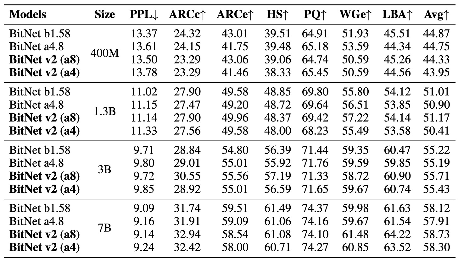
Perplexity and results of BitNet v2, BitNet a4.8 and BitNet b1.58 on the end tasks. Inspite of all the optimizations during forward pass, according to me the paper still lacks innovation in backward pass, where they used STEs instead of maybe an improved version of DGEs.
During the error propagation and gradient calculation, the authors stayed with usage of Activation clamping, which as the 4-bit training paper shows is not a good thing, hence, they should have employed something like a sparse residual matrix as loss for next layer.
BitNetv2 also doesn’t explore using teacher-student frameworks to further improve low-bit student performance, which could have boosted the performance by some margin (though it is understandable, as the major attempt of the paper is to show that this methodology works).
In my opinion, instead of using backprop based gradient estimates, why not try forward-forward type estimations, ultra-low precision types serves as best grounds for doing the optimization (as we need to worry about significance of grads while updation), also we are spared from computing gradients through things like STEs or DGEs.
Conclusion
In this unapologetically long article, we started from gently introducing the topic of low precision training. From there we tried to figure out how is 1-bit training final frontier and advantages it provides. Then we saw issues with 1-bit models and the first attempt in the direction (BitNet), then we discussed the available improvements over BitNet and how BitNet v2 lunged forward to handle it. Finally we went through few components in greater detail and then discussed about results and outcomes of the overall methodology. With my final thoughts over further improvement we concluded the article.
I hope this article helps in understanding the idea behind ultra-low precision models and hence, convinces you in start exploring and contributing on these topics.
I will encourage you to refer to the paper and go through the references in great details to have more fine-grained understanding.
BitNet : https://arxiv.org/abs/2310.11453
BitNet v2 : https://arxiv.org/pdf/2504.18415
That's all for today.
Follow me on LinkedIn and Substack for more such posts and recommendations, till then happy Learning. Bye👋
Shouldnt 1 bit only have two possible values? 1.58 bit gives 3 possible values.