Decoding Logistic Regression: From Lines to Probabilities

Discover how a simple twist on Linear Regression unlocks the power of classification, and dive into the mechanics of the Sigmoid function and the Log-Loss cost function.

Table of content

1. Introduction: The Next Frontier is Classification

2. The Problem: Why a Straight Line Fails at "Yes" or "No"

3. The Solution: The "S"-Shaped Sigmoid Function

4. How Do We Measure Error in a Game of Probabilities?

5. The Strategy: The Familiar "Downhill Walk"

6. Deep Dive: The Math of Logistic Regression's Gradient

7. Going Deeper: Calculate the Probabilities with the Vizuara AI Learning Lab!

8. Conclusion

1. Introduction: The Next Frontier is Classification

Think about the questions we ask every day. Many of them have numerical answers. "What will the temperature be tomorrow?" "How much will this house cost?" "How many points will my team score?" In our last blog, we explored Linear Regression, a powerful tool for teaching a machine to answer exactly these kinds of questions to predict a continuous, numerical value.

But there's a whole other universe of questions we face. A fundamentally different kind. These are the "yes or no," the "this or that" questions. "Will this customer cancel their subscription?" "Is this email spam or not?" "Does this patient have the disease?" The answer isn't a number on a sliding scale; it's a distinct category, a label, a choice.

What if we could teach a machine to make these categorical decisions? What if we could give it a set of data and empower it to draw a line, not to predict a value, but to separate two different groups? This is the fundamental quest of classification, one of the most important pillars of machine learning. And our first, most essential tool for this task is an algorithm with a slightly misleading name: Logistic Regression.

Despite its name, Logistic Regression is our go-to method for classification. Its primary purpose is to answer a powerful new kind of question: "Given this set of information, what is the probability that it belongs to a certain category?"

By learning to calculate these probabilities, a machine can make remarkably sophisticated decisions. It's the core technology behind countless systems you interact with daily, from your bank's fraud detection system flagging a suspicious transaction to a doctor's diagnostic tool assessing the likelihood of a tumor being malignant. It's the engine that decides whether to approve a loan or filter an email.

Just like its linear cousin, this technique comes in a couple of key flavors.

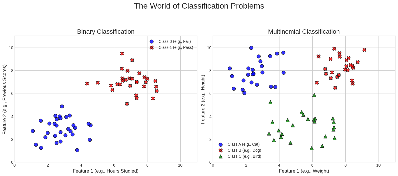
Binary Classification: This is the most common form, where we are predicting between exactly two outcomes (Yes/No, 1/0, Spam/Not Spam). This will be our focus for this blog.

Multinomial Classification: This is an extension that handles problems with three or more categories, like classifying a news article as "Sports," "Politics," or "Technology."

In this article, we're going to pull back the curtain on Binary Logistic Regression. We'll discover why a simple straight line fails spectacularly at this new task. We'll explore the hidden mechanics of the "S"-shaped Sigmoid function that makes classification possible. We'll uncover a brand-new way to measure error with a powerful cost function, and we'll see how our old friend, the "downhill walk" of Gradient Descent, can be used to master this new landscape.

2. The Problem: Why a Straight Line Fails at "Yes" or "No"

Our new mission is to build a classification model. Let's ground this in a simple, intuitive example. Imagine we have data on students from a programming course. We have two columns: the number of hours each student studied and a simple binary outcome whether they passed the final exam (which we'll represent as 1) or failed (which we'll represent as 0).

Our task is to build a model that, given the hours a new student studies, can predict whether they will pass or fail.

As always, our first step is to visualize the data. Let's plot "Hours Studied" on the x-axis and the "Pass/Fail" outcome on the y-axis.

Looking at this plot, the relationship is clear. Students who study for fewer hours tend to fail (y=0), and students who study for more hours tend to pass (y=1). There's a clear separation.

So, being familiar with our previous tool, a natural first thought might be: "Why don't we just use Linear Regression? Let's find the best-fit line for this data!"

Let's try it and see what happens.

By fitting this line, we've immediately run into two huge, deal-breaking problems:

Problem 1: The Output Isn't a Probability

Remember, for classification, we want to predict the probability of an outcome. A probability must be between 0 and 1. But as you saw in the animation, the straight line doesn't care about these boundaries. It happily extends upwards past 1 and downwards below 0.

What does a "150% probability of passing" mean? Or a "-20% probability of passing"? Nothing. They are complete nonsense. Our model is producing outputs that are fundamentally invalid for the problem we're trying to solve. We need a function that is "squashed," one that can never go above 1 or below 0.

Problem 2: It's Incredibly Sensitive to Outliers

Let's say we add one more data point to our set: a student who studied an exceptionally long time (e.g., 20 hours) but still passed. This is an outlier, but a valid piece of data. Let's see what happens to our best-fit line.

Look at that! A single outlier has dragged our entire line to the right. This shift can completely change our model's predictions. Let's say we set a rule: "If the line's prediction is > 0.5, we predict 'Pass'; otherwise, we predict 'Fail'." The point where the line crosses this 0.5 threshold is our decision boundary.

Because of that one outlier, our decision boundary has shifted. Now, a student who might have been classified as "Pass" with the old line might be classified as "Fail" with the new one. Our model is not robust; it's easily thrown off by new data.

It's clear that Linear Regression is the wrong tool for the job. We can't use a model that produces unbounded, nonsensical values and is so easily swayed by outliers. We need a new kind of model. We need a line that doesn't go on forever, we need a line that gracefully bends into an 'S' shape, perfectly constrained between 0 and 1.

3. The Solution: The "S"-Shaped Sigmoid Function

Our traditional Linear Regression model, with its unbounded straight line, simply cannot handle the binary world of "yes" or "no." We need a mathematical superhero, a function that can take any continuous numerical input, no matter how large or how small, positive or negative and elegantly squash it into a value that always falls strictly between 0 and 1. This "squashed" output can then be directly interpreted as a probability.

Enter the Sigmoid function, also known as the Logistic function. This is the core innovation that transforms a linear model into a powerful classification engine. Its elegance lies in its simplicity and its perfectly "S"-shaped curve.

The mathematical formula for the Sigmoid function is:

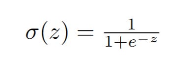
Let's break down this formula piece by piece:

z: This represents any real number input. In the context of Logistic Regression, this z is exactly what our Linear Regression equation would normally output: z = (m * x) + b. So, z is our weighted sum of inputs plus the bias. It’s often referred to as the logit or log-odds.

e: This is Euler's number, a fundamental mathematical constant approximately equal to 2.71828. It's the base of the natural logarithm and appears naturally in many growth and decay processes.

-z: Notice the negative sign in the exponent. This is crucial for the 'S' shape. As z becomes very large and positive, -z becomes very large and negative, causing e^-z to approach zero. As z becomes very large and negative, -z becomes very large and positive, causing e^-z to become a very large number.

Now, let's visualize this beautiful curve and understand its magical properties:

Observe the shape. It's a smooth, continuous curve that resembles an 'S'. This unique form is precisely what we need:

1. Bounded Output (0 to 1): No matter what value z takes – whether it's -100, 0, or 1000 – the Sigmoid function will always output a value between 0 and 1.

   • If z is a very large negative number (e.g., -100), e^-z becomes an extremely large positive number, making the denominator (1 + e^-z) huge. Consequently, 1 / (huge number) approaches 0.

   • If z is a very large positive number (e.g., 100), e^-z becomes an extremely small positive number (approaching 0). This makes the denominator (1 + e^-z) approach 1. Consequently, 1 / 1 approaches 1.

   • If z is exactly 0, e^-0 is e^0 = 1. So, σ(0) = 1 / (1 + 1) = 1 / 2 = 0.5. This point, where the S-curve crosses 0.5, is incredibly important.

2. Probability Interpretation: Because its output is always between 0 and 1, we can legitimately interpret σ(z) as the probability of the positive class (e.g., the probability of a student passing the exam). A prediction of 0.8 means an 80% chance of passing, and a prediction of 0.2 means a 20% chance. This instantly solves Problem 1 from our previous section.

3. Non-Linearity: Unlike Linear Regression, which is strictly linear, the Sigmoid function introduces a crucial element of non-linearity. This S-shape allows the model to capture more complex relationships in the data, making it suitable for separating classes that aren't neatly divided by a straight line.

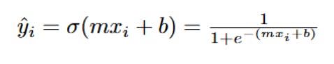
Now, let's connect this back to our original linear model. In Logistic Regression, we don't directly predict y = (m * x) + b. Instead, we take the output of that linear combination and feed it into the Sigmoid function. So, for our "Hours Studied" example:

This means:

1. We still calculate a linear score (m * HoursStudied + b), but this score is not our final prediction.

2. This linear score (our z) is then transformed by the Sigmoid function into a probability P(Pass) that is always between 0 and 1.

3. A high linear score (large positive z) will result in a high probability (close to 1), indicating a high likelihood of passing.

4. A low linear score (large negative z) will result in a low probability (close to 0), indicating a low likelihood of passing.

Finally, once we have these probabilities, we need a rule to make a definitive "Yes" or "No" classification. This is where the decision boundary comes in. Typically, for binary classification, we use a threshold of 0.5:

If P(Pass) ≥ 0.5, we classify the student as "Pass" (1).

If P(Pass) < 0.5, we classify the student as "Fail" (0).

Remember how z=0 results in σ(z)=0.5? This means our decision boundary of P(Pass)=0.5 directly corresponds to the point where our linear combination (m * HoursStudied + b) equals 0. In the input space, m * HoursStudied + b = 0 defines the straight line that separates our "Pass" predictions from our "Fail" predictions. This elegantly solves the outlier sensitivity issue by ensuring that probabilities never go out of bounds, no matter how extreme an outlier's x value might be. The S-curve might get steeper or flatter, but it will always remain constrained between 0 and 1, making our decision boundary more robust.

4. How Do We Measure Error in a Game of Probabilities?

With Linear Regression, our life was relatively simple when it came to measuring error. We calculated the squared difference between the actual value and the predicted value for each point, summed them up, and took the average. This gave us our Mean Squared Error (MSE), and its beautiful, bowl-shaped landscape allowed Gradient Descent to reliably find the perfect m and b.

Now, we've introduced the Sigmoid function into our model:

Our model now outputs a probability ŷ between 0 and 1. This is fantastic for interpretation! But here's the crucial question: Can we still use MSE as our cost function? Let's quickly re-evaluate:

Here yi,is either 0 or 1, and ŷi is the probability output by the Sigmoid function. It might seem logical to continue using MSE, as it still measures the "distance" between our prediction and the truth. However, when we combine the Sigmoid function with MSE, something goes terribly wrong.

The Hidden Flaw: Non-Convexity

The biggest problem with using MSE for Logistic Regression is that it creates a non-convex cost function.

Remember our beautiful 3D landscape from the Linear Regression post, where the cost function was a smooth, upward-curving bowl? That smooth bowl is called a convex function. A convex function has one fantastic property: it has only one global minimum. No matter where Gradient Descent starts on that landscape, it will always slide down to the very bottom of the bowl and find the absolute best m and b.

When you plug the Sigmoid function into the MSE formula, the resulting cost function landscape for m and b becomes bumpy and riddled with many local minima. It's no longer a smooth bowl. Imagine trying to find the lowest point in a vast, mountainous region, but every time you go downhill, you might just end up in a small dip (a local minimum) that isn't the true lowest point of the entire region (the global minimum).

If our Gradient Descent algorithm gets stuck in one of these "local minima," it means it will find an m and b that represents a good fit, but not necessarily the best possible fit for our data. Our model would be suboptimal, and we'd never know if we could have done better. This is a deal-breaker for a reliable machine learning model.

So, we cannot use MSE. We need a different cost function. One that, when combined with the Sigmoid function, results in a convex optimization problem. This ensures that Gradient Descent can always reliably find the single global minimum, giving us the truly optimal m and b.

The Solution: Log-Loss (Binary Cross-Entropy)

The answer to this problem is a powerful and elegant cost function called Log-Loss, also widely known as Binary Cross-Entropy (BCE). This function is specifically designed for classification problems where the model outputs probabilities.

Log-Loss works by penalizing the model much more severely when it is confidently wrong. Conversely, it rewards the model by assigning a very small penalty when it is confidently correct.

Let's break down the intuition behind this. The Log-Loss function has two main parts, one for each possible true outcome (since our y_i can only be 0 or 1):

Case 1: When the Actual Outcome is 1 (Positive Class, e.g., Student Passed)

If the student actually passed (yi = 1) we want our model ŷi to predict a probability as close to 1 as possible.

The loss for this single data point is given by:

Let's think about what happens with this formula:

• If the model is correct and confident: It predicts ŷi = 0.99. The loss is -log(0.99), which is a tiny number (around 0.01). The penalty is very small. Good job, model.

• If the model is unsure: It predicts y_hat = 0.5. The loss is -log(0.5), which is a moderate number (around 0.69). The penalty is noticeable.

• If the model is wrong and confident: It predicts y_hat = 0.01 (a 1% chance of passing), but the student actually passed. The loss is -log(0.01), which is a huge number (around 4.6). The penalty is massive. Log-Loss severely punishes the model for being so sure of the wrong answer.

The negative logarithm creates a curve that explodes towards infinity as the prediction approaches 0, and smoothly goes to 0 as the prediction approaches 1.

This handles the case where the true answer is 1. But what about when the true answer is 0?

Case 2: The real answer is 0 (e.g., the student Failed)

If the student actually failed (the true y is 0), we want our model's predicted probability (y_hat) to be as close to 0 as possible. The loss for this case is calculated with a slightly different formula:

Let's trace the logic here:

• If the model is correct and confident: It predicts ŷi = 0.01. Then (1 - ŷi) is 0.99. The loss is -log(0.99), which is a tiny number (around 0.01). The penalty is very small.

• If the model is unsure: It predicts ŷi = 0.5. Then (1 - ŷi) is 0.5. The loss is -log(0.5), which is a moderate number (around 0.69).

• If the model is wrong and confident: It predicts ŷi = 0.99 (a 99% chance of passing), but the student actually failed. Then (1 - ŷi) is 0.01. The loss is -log(0.01), which is a huge number (around 4.6). Again, the penalty is massive for being confidently wrong.

This second function creates a mirror image of the first. It explodes towards infinity as the prediction approaches 1 and goes to 0 as the prediction approaches 0.

We now have two brilliant functions, one for each possible outcome. But how do we combine them into a single cost function that works for all our data points at once? That's the next piece of the puzzle.

Putting It All Together: The Single Log-Loss Equation

So, we have two separate loss functions:

• If y = 1, our loss is -log(ŷi)

• If y = 0, our loss is -log(1 - ŷi)

Having to switch between two different formulas depending on the true value of y is clumsy. We need a way to express this in a single, unified equation. The machine learning community came up with a very clever mathematical trick to do just that.

Here is the combined Log-Loss equation for a single data point:

Let's see why this brilliant piece of math works perfectly. Remember that our true value, y, can only be 1 or 0.

• Consider the case where the true value is y = 1:

  • The first part of the equation becomes 1 * log(ŷ), which is just log(ŷ).

  • The second part becomes (1 - 1) * log(1 - ŷ), which is 0 * log(1 - ŷ) = 0.

  • So, the entire equation simplifies to Loss = - [ log(ŷ) + 0 ] = -log(ŷ). This is exactly the formula we wanted for the y=1 case!

• Now, consider the case where the true value is y = 0:

  • The first part of the equation becomes 0 * log(ŷ) = 0.

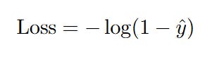
  • The second part becomes (1 - 0) * log(1 - ŷ), which is 1 * log(1 - ŷ) = log(1 - ŷ).

  • So, the entire equation simplifies to Loss = - [ 0 + log(1 - ŷ) ] = -log(1 - ŷ). This is exactly the formula we wanted for the y=0 case!

This single equation elegantly handles both scenarios. It uses the value of the true y to "turn on" the correct part of the loss function and "turn off" the other part. It's a compact and powerful way to write our loss logic.

The Final Cost Function

We're now in the home stretch. The equation above gives us the loss for a single data point. To get the total cost for our entire dataset, we do exactly what we did for Linear Regression: we sum up the individual losses for all n data points and then take the average to get the final cost.

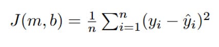
This gives us the complete Cost Function for Logistic Regression, J(m, b):

Let's break down this final formula:

• J(m, b): Just like before, the cost J is a function of our model's parameters, m and b. Changing m or b changes our predictions (ŷ), which in turn changes the total cost.

• - (1/n): We average the loss over all n data points. The negative sign is part of the Log-Loss definition we established.

• Σ [ ... ]: This is the "sum over all data points" of the clever single-point loss function we just derived.

We have now successfully defined our new mission. We've left the bumpy, non-convex world of MSE behind and arrived at a new, smooth, convex cost function, Log-Loss.

Our objective is once again clear and precise: find the specific values of m and b that minimize this new cost function, J(m, b).

And the strategy to achieve this? It's our reliable, old friend: Gradient Descent.

5. The Strategy: The Familiar "Downhill Walk"

Our journey has led us to a crucial point. We have a new problem (classification), a new model that outputs probabilities (the Sigmoid function), and a new way to measure error that is specifically designed for these probabilities (the Log-Loss cost function). We have successfully engineered a cost function, J(m, b), that creates a smooth, convex, bowl-shaped landscape. This means there are no tricky local minima to fall into—only one single, true global minimum.

So, how do we find the bottom of this new bowl? How do we find the perfect duo of m and b that gives us the absolute minimum possible Log-Loss?

The answer should feel like meeting an old friend in a new city. The strategy is exactly the same one we mastered with Linear Regression: Gradient Descent.

The intuition is identical, and it's worth revisiting because it's so powerful. We imagine our new Log-Loss cost function as a physical, 3D landscape.

• The two horizontal axes still represent every possible value for our parameters, m and b.

• The vertical height at any point still represents the Cost (J) for that specific combination of m and b. A higher point means our model is making worse predictions and has a higher Log-Loss.

• The absolute lowest point in this landscape is still our global minimum. This point represents the specific m and b that make our Logistic Regression model as accurate as it can possibly be.

Our method for finding this lowest point is the same "downhill walk" algorithm:

1. Start Somewhere Random: We begin by initializing m and b to some starting values, often just zero. This is like dropping a ball at a random point on the side of our 3D hill.

2. Find the Steepest Downhill Direction: This is the core of the algorithm. From our current position (m_old, b_old), we need to figure out which way is "down." To do this, we calculate the gradient of our new Log-Loss cost function. The gradient is still a vector of two partial derivatives:

   • ∂J/∂m: How does the Log-Loss change if we nudge m?

   • ∂J/∂b: How does the Log-Loss change if we nudge b?
     This gradient vector tells us the direction of steepest ascent (uphill). Therefore, the fastest way downhill is, once again, the opposite direction of the gradient.

3. Take a Small Step: We update our parameters by taking a small step in that downhill direction. The size of this step is controlled by our Learning Rate (α), a small number we choose (like 0.01).

4. Repeat, Repeat, Repeat: We are now at a new, slightly lower point on the hill. We repeat the entire process: calculate the new gradient from this new spot, and take another small step downhill.

We continue this iterative process calculate gradient, update parameters, calculate gradient, update parameters hundreds or thousands of times. With each step, m and b get closer and closer to their optimal values. Our model's predictions get better, and the Log-Loss cost gets smaller.

Eventually, our steps will become infinitesimally small as we reach the flat bottom of the valley. At this point, we have converged. The final m and b values are the ones that define our best-fit classification model.

The beautiful thing is that the high-level strategy hasn't changed at all. The only thing that's new is the specific landscape we're walking on. This means our only remaining task is a familiar one: we need to roll up our sleeves, dive into the calculus, and figure out the exact mathematical formulas for the partial derivatives of our new Log-Loss cost function.

6. Deep Dive: The Math of the Gradient for Log-Loss

We have our strategy: use Gradient Descent. We have our update rules:

Now, we must derive the formulas for those two partial derivatives, ∂J/∂m and ∂J/∂b, using our new Log-Loss cost function. This derivation is one of the most beautiful and surprising in all of introductory machine learning. It looks much more intimidating than it is, and the final result will be very satisfying.

Step 1: Setting up the Full Equation

First, let's write out our full Log-Loss cost function, J(m, b). We need to substitute the definition of y_hat (our prediction) directly into the equation.

Remember:

So, the full cost function is:

This is the beast we need to differentiate. We'll do it piece by piece using the Chain Rule, focusing first on how the cost J changes with respect to the slope m.

Step 2: Calculating the Gradient for the Slope (∂J/∂m)

To find ∂J/∂m, we can ignore the (1/n) and the summation Σ for a moment and just focus on the loss for a single data point i. Then we'll add the summation and averaging back in at the end.

The loss for a single point is:

We need to find ∂(Loss_i)/∂m. Since the two terms are added together, we can differentiate them separately:

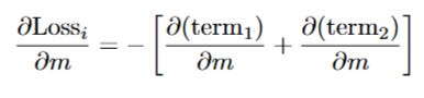
Let's do this one term at a time.

Differentiating the first term: yi * log(ŷi)

Here, yi is a constant (either 0 or 1), so we just need to find the derivative of log(ŷi). This requires the Chain Rule.

Now we need to find ∂(ŷi)/∂m. Remember, ŷi = sigmoid(z_i). So we use the Chain Rule again!

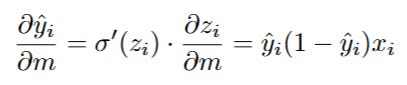
A very useful property of the Sigmoid function is that its derivative is simply sigmoid(z) * (1 - sigmoid(z)). Since ŷ = sigmoid(z), the derivative is just y_hat * (1 - y_hat).

The derivative of z_i = m*x_i + b with respect to m is just x_i.

So,

Let's substitute this back into our log derivative:

The ŷi in the numerator and denominator cancel out! This leaves us with:

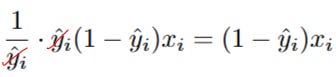
So, the full derivative of the first term is yi * (1 - ŷ) * xi.

Differentiating the second term: (1 - yi) * log(1 - ŷi)

This is very similar. (1 - yi) is a constant. We use the Chain Rule for log(1 - ŷi):

The derivative of (1 - ŷi) with respect to m is 0 - ∂(ŷi)/∂m.

We already found ∂(ŷi)/∂m above! It's ŷi * (1 - y_hat_i) * x_i.

So,

Let's substitute this back in:

So, the full derivative of the second term is

Putting it all together for one data point

Now we combine the derivatives of our two terms:

Let's expand and simplify this. We can factor out the common xi term.

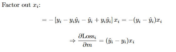
The Final Gradient for m

This is the derivative for just one data point. To get the final gradient for the whole cost function, ∂J/∂m, we just put the summation and the -(1/n) factor back in. (Note: the minus sign from -(1/n) will flip our (ŷi - yi) term).

Now, we apply this to the full cost function J(m, b) = (1/n) * Σ (Loss_i).

This is a stunning result. After all that complex differentiation with logs and sigmoids, the final formula for the gradient with respect to m looks remarkably clean. It's simply the average of the error (y_hat - y) multiplied by the input x for each data point.

Step 3: Calculating the Gradient for the Intercept (∂J/∂b)

Now we find the gradient for b. The process is identical, but the calculus is simpler. We start with the derivative of the single-point loss with respect to b.

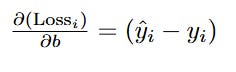
(Wait, how did we get that so fast?)

Let's quickly trace the Chain Rule. The derivative of z = mx + b with respect to b is just 1. All the other complex parts of the derivative cancel out in exactly the same way as before, but this time they are multiplied by 1 instead of by x_i. This leaves us with just the core error term.

Now, to get the final gradient for our entire cost function J, we simply take the average of this error term across all our n data points.

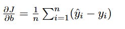
And that's it. It's simply the average of the prediction error.

Step 4: The Final Update Rules - A Moment of Shock and Awe

Let's write our two final gradient formulas side-by-side:

Now, take a moment. If you look back at our Linear Regression post, these formulas are structurally identical to the gradients we derived for Mean Squared Error.

This is a stunning result. We used a completely different model (Sigmoid) and a completely different cost function (Log-Loss), yet the final update rules for Gradient Descent came out looking the same. This isn't a coincidence; it's a result of deep mathematical elegance.

The only thing that has changed is how we calculate the prediction ŷ:

• In Linear Regression: ŷ = m*x + b

• In Logistic Regression: ŷ = sigmoid(m*x + b)

Once you have that prediction ŷ, the process for calculating the gradients and updating m and b follows the same powerful structure. This beautiful consistency is one of the reasons these concepts are so fundamental to all of machine learning.

7. Going Deeper: Calculate the Probabilities with the Vizuara AI Learning Lab!

We have journeyed from the simple idea of a "yes or no" question all the way through to the calculus of the Log-Loss function. But to truly make these concepts stick, you have to get your hands dirty with the numbers.

That's why we've built the next part of our interactive series. This isn't a simulation to just watch; it's a hands-on environment where you become the learning algorithm. You will step through the core calculations of Logistic Regression yourself to see how a machine learns to predict probabilities.

In this lab, you will:

• Calculate Sigmoid Outputs: Manually plug the linear score (z = mx + b) into the Sigmoid function to see how it's squashed into a probability.

• Compute Log-Loss: Experience firsthand how the cost function heavily penalizes a confident but wrong prediction.

• Derive the Gradients: Use the formulas we just derived to calculate the exact gradients for m and b for a given step.

• Connect Theory to Practice: Solidify your understanding by bridging the gap between the abstract formulas and the concrete numbers that drive the learning process.

Reading about a concept is knowledge. Calculating it is understanding.

Ready to get your hands dirty? Visit the Vizuara AI Learning Lab now!

---

8. Conclusion

We started our journey with a new kind of problem, a world of "yes or no" questions where our old tools failed us. We saw how a simple straight line from Linear Regression couldn't handle the task of classification, producing nonsensical predictions and being easily swayed by outliers.

Then came the brilliant idea: the Sigmoid function. We saw how this elegant 'S'-shaped curve could take any number and gracefully squash it into a valid probability between 0 and 1, giving our model the power to speak the language of likelihood.

But this new model required a new way to measure "wrongness." We discovered that our old friend, Mean Squared Error, created a treacherous, bumpy landscape. So we introduced a new Cost Function, Log-Loss, which is perfectly designed for probabilities and punishes a model most when it is confidently wrong.

Finally, we unveiled the strategy to conquer this new landscape: our trusted algorithm, Gradient Descent. We learned the beautiful intuition of "walking downhill," and we dove into the calculus to derive the exact formulas that guide every step. In a moment of beautiful mathematical symmetry, we discovered that the final gradient formulas were structurally identical to those from Linear Regression.

In essence, you now understand the complete story of how a machine learns to classify. It starts with a model that produces probabilities (Logistic Regression), measures its performance with a cost function designed for those probabilities (Log-Loss), and then iteratively improves that model using an optimization algorithm (Gradient Descent).

You've decoded the absolute foundation of classification. This core concept of transforming a linear output into a probability is the very same principle used in the final layers of massive neural networks that decide whether an image contains a cat or a dog. You've mastered another fundamental building block of modern AI.

So.. that's all for today.

Follow me on LinkedIn and Substack for more such posts and recommendations, till then happy Learning. Bye👋