
Speculative Decoding — Think Fast⚡, Then Think Right✅
Can two LLMs be faster than one? Exploring Speculative decoding : An ingenious method to leverage benefits form Large LMs and small LMs to mitigate their respective bottlenecks.

Table of content
Introduction
Problems with Current AR Models
Insights: What Should Happen Ideally?
Methodology
Components
Algorithm
A Quick mathematical analysis
Usage
Thoughts
Conclusion
Introduction
What if we could make large language models think faster, without sacrificing their brilliance?
Enter speculative decoding — an approach that promises just that: speeding up large model inference by combining the best of both worlds (fast small models + accurate big ones). The core idea? Let the small model guess, and the big model verify (and sometimes correct).
But before diving into that, let’s quickly revisit what drives all of this — the good old auto-regressive models.
Auto-Regressive (AR) language models work by predicting one token at a time, each step conditioned on everything generated so far. It's like writing a story word by word, making sure each new word fits in with what you've already written. This sequential nature, while intuitive, is also the bottleneck. Why? Let’s understand.
Problems with Current AR Models
AR (Auto-regressive) models don't directly spit out text. First, they generate a probability distribution over the entire vocabulary for the next token. Then they sample one token from this distribution (though deterministic algorithms like beam-search, greedy-search, top-k. etc). This two-step dance though gives more flexibility but adds latency, especially when repeated thousands of time as the generation of next token is directly dependent on previous sampled token (not the PDF over the vocab). This means if you want to generate 100 words, then you will repeat the process of pdf generation and sampling 100 times. This results in computational and time bottlenecks as soon as we start talking about very Large models like LLMs.
The entire existence of tokens in PDF and then sampling to make token deterministic feels a bit like quantum physics ⚛️
Just like an electron exists in a probabilistic cloud until it's observed (i.e. sampled), a token in an LLM isn't "real" until it's sampled. The model holds a probability distribution — the quantum fog — and then collapses it to one token — the classical result. This quantum-style uncertainty is cool, but computationally expensive.
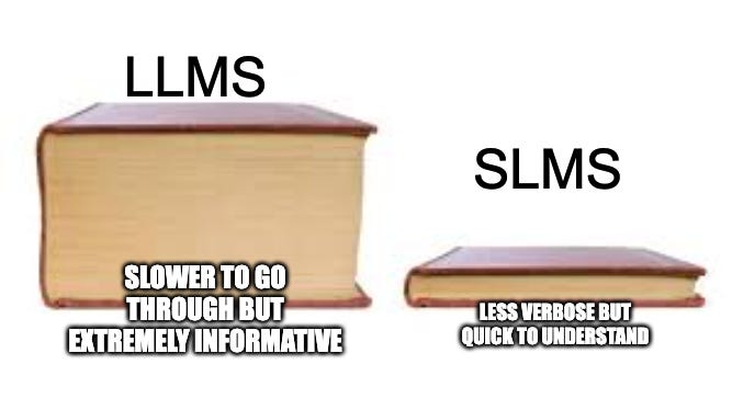
Bigger models: pros and cons
Larger models like GPT-4, Gemini, or Claude 3 offer incredible fluency and reasoning. But they:
Are slow to generate (high compute cost)
Consume more memory
Often overkill for simpler next-token predictions (like predicting “.” after a sentence)
Smaller models: pros and cons
Tiny models (like distilled transformers, or older 1-2B models):
Are blazingly fast
Consume less memory
But, they fail in long-form reasoning or ambiguous next-token cases
So what if we combine the two in a smart way? 🤔
Insights: What Should Happen Ideally?
Not all tokens are equal. Some are easy to guess (like punctuation, common stopwords, prepositions), while others are harder (like domain-specific jargon, rare idioms, etc.).
So ideally:
Small models should handle easy tokens — they’re fast and good enough for that.
Big models should only intervene when necessary — like a strict professor double-checking a junior’s work.
This is exactly what speculative decoding does.
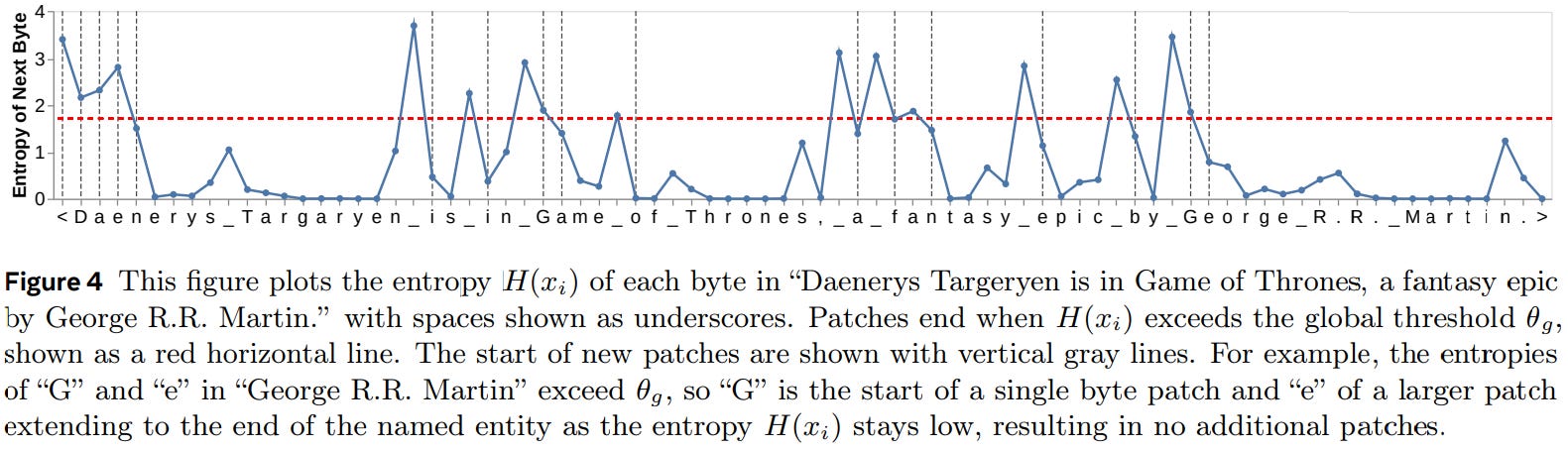
In one of our previous article on Byte Latent Transformers (BLT) we discussed an entropy-based view where tokens with lower entropy (i.e. high confidence) are easier and should be treated differently from those with higher entropy (i.e. uncertain predictions). We’ll borrow a similar intuition here.
Methodology
(The video above is taken from https://research.google/blog/looking-back-at-speculative-decoding/ and explain very beautifully the procedural generation of speculative decoding)
Before diving into the algorithm itself let's get some clarity over the components.
Components
1. Draft model : The smaller model serves as a helper/assistant to the larger model. The draft model could be any model with similar input-output space and is really fast, though the target functionality could be anything, imagine a draft model which is slow but specializes in generating reasoning tokens or something.

2. Target model : The target model is sort of validator which evaluates and accepts (or rejects) the guesses. If a certain guess doesn't follow the criterion (which we will discuss below) then the sample is rejected and is replaced by the target models prediction.

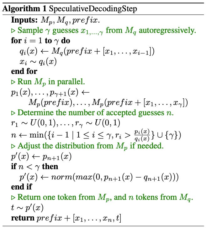
Algorithm
(we will closely follow the algo mentioned in the image below)
Step 1 : Drafting Phase
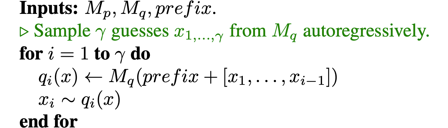
The process begins with the draft model (P) generating a sequence of potential tokens of length K (given as [gamma] in paper, based on the given initial context. For instance, consider the context "The future of AI is". The draft model might propose the continuation " promising and full of potential". Along with the set of tokens we also get the probability distribution for each token which we store.
Step 2 : Verification Phase
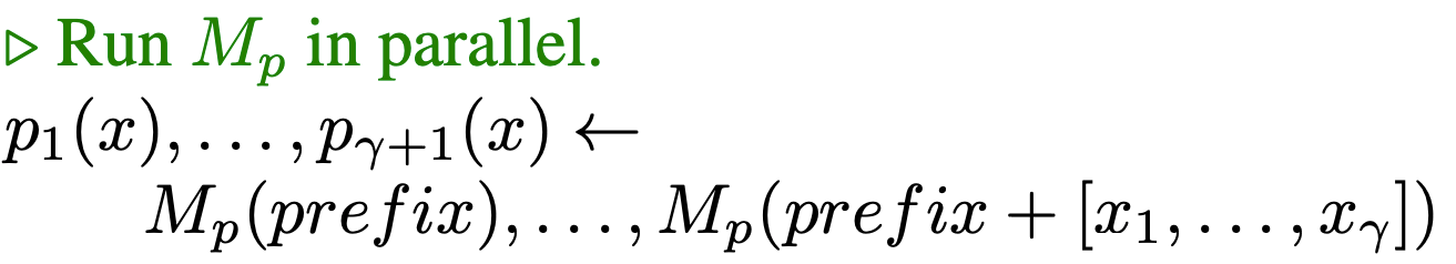
The target model (Q)
takes in the sequence generated by draft model as input and then through a single forward pass predicts the probability of each token in sequence. Along with that it predicts the probability of next token in vocab (k+1th).
Step 3 : Correction phase
For every single tokens probability which we get from draft model (P) we compare it index by index against the pdf given by target model (Q) based on the formula below
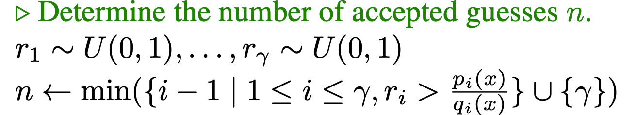
The first index where the probability vector from draft model is lower than the probability vector from target model of that token serves as the breakage point. The entire sequence from T to T+N is omitted and the sequence from 0 to T-1 is moved to final output. Along with that the target model also then samples the next token from pdf that we have already predicted in the forward pass.
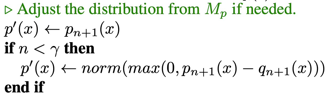
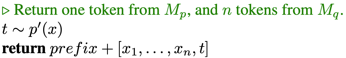
Step 4 : Re-assignment
The initial sequence is updated with the output sequence and then process repeats till we reach end of sequence.
Now we know each component lets look at the combined picture. Here
Mp : Target model (Bigger)
Mq : Draft model (smaller)
prefix : initial token sequence
γ : Number of tokens to generate by draft model (Mq)
P(x) : Probability of selected token from Target model (Mp)
Q(x) : Probability of selected token from draft model (Mq)
A quick mathematical analysis
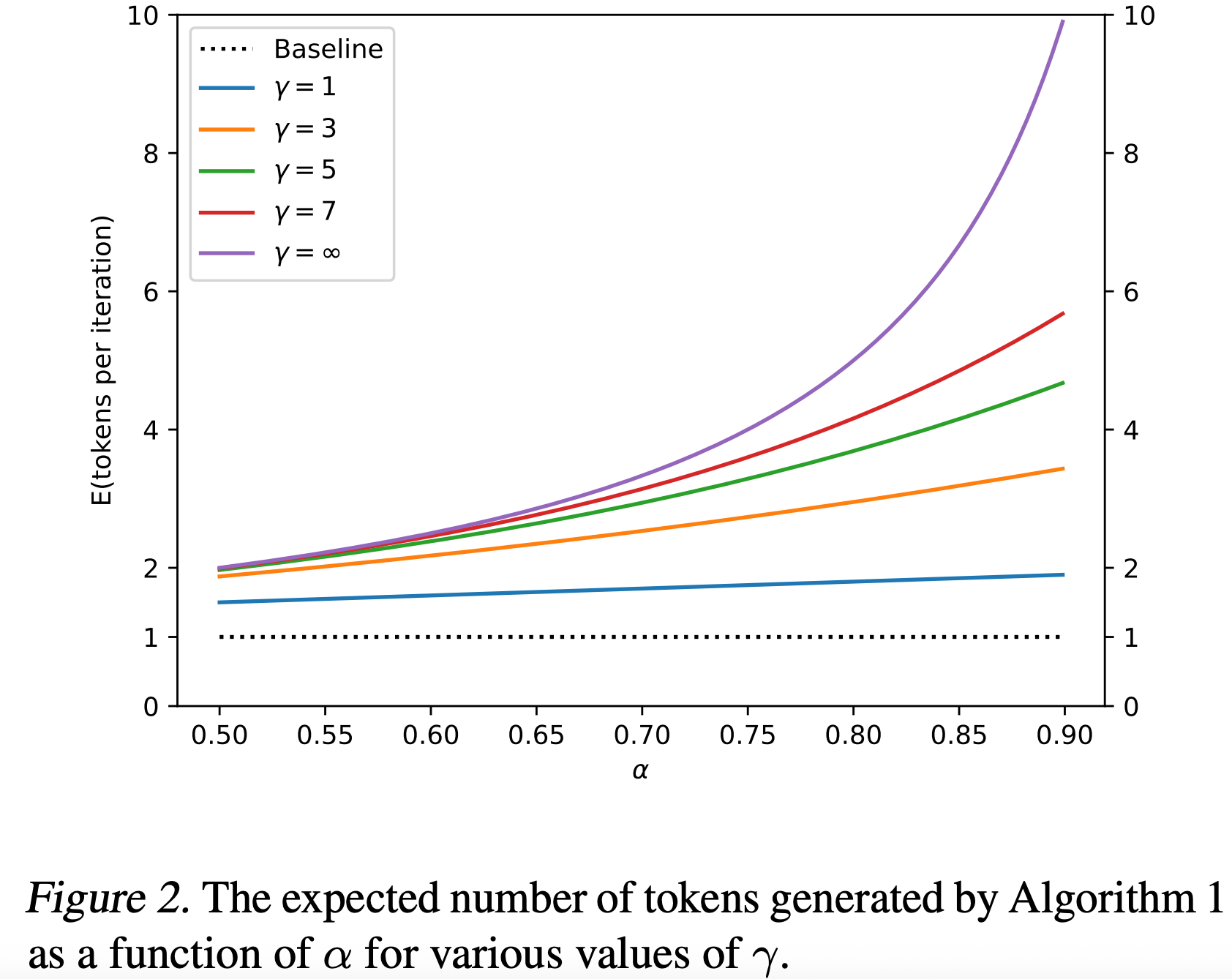
The acceptance rate of the sequence suggested by draft model is given by β, and E(β) or Expectation of β is then a natural measure of how well Mq approximates Mp. This means that expected number of tokens predicted by the entire process flow we discussed above could be defined as (If we make the simplifying assumption that the βs are i.i.d., and denote α = E(β) by this geometric relation,
Authors also gave the proof that in ideal case the distribution P and Q where they prove that α is equivalent to inverse of average divergence seen between P and Q distribution (being modelled by target and draft model) that by minimizing the natural divergnce (which is symmetric, similar to Jensen-Shannon Divergence) they can increase the average number of predicted tokens in a single pass.
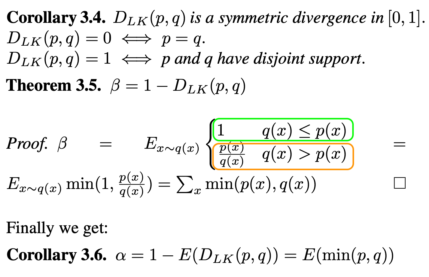
In proof, the selection condition is highlighted in orange, which basically says that the probability of rejection of suggested tokens by draft models is given by p(x)/q(x) which is 1 when q(x) < p(x), and inverse of this expectation over this divergence in probability gives the α (which is acceptance). Example, if draft model (q) predicted 5 tokens such that probability of each is equal or higher than the prediction from target model then α=1 as the D(p, q) = 0 (also depicted in the graph above) and by the formula mentioned above defining geometric relation between α and E(# of tokens generated) we can see number of tokens per iteration increase (governed by γ which is a heuristic).
Usage
The simplest implementation source I found is by using the HuggingFace transformers pipeline. The draft model here is referred to as “assistant model” and the target model is referred by “model”. See the snapshot below to understand how easy the setup is. Also checkout this (Dynamic speculation).

Thoughts
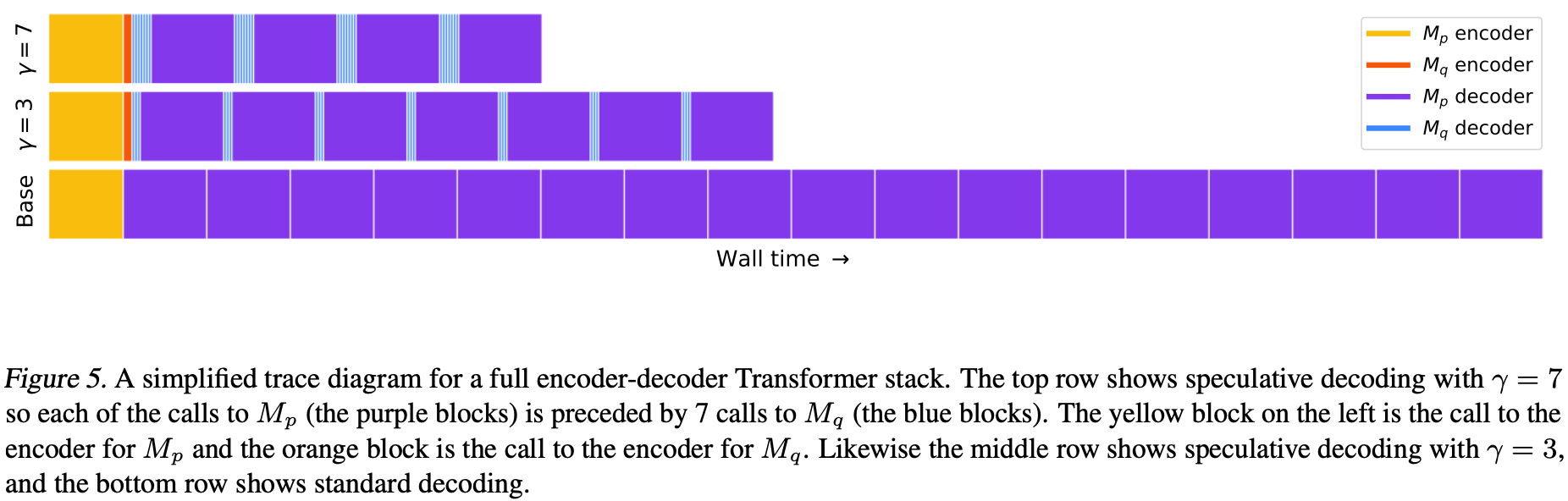
Much shorter wall time as compared to usage of full target model. See the diagram below.
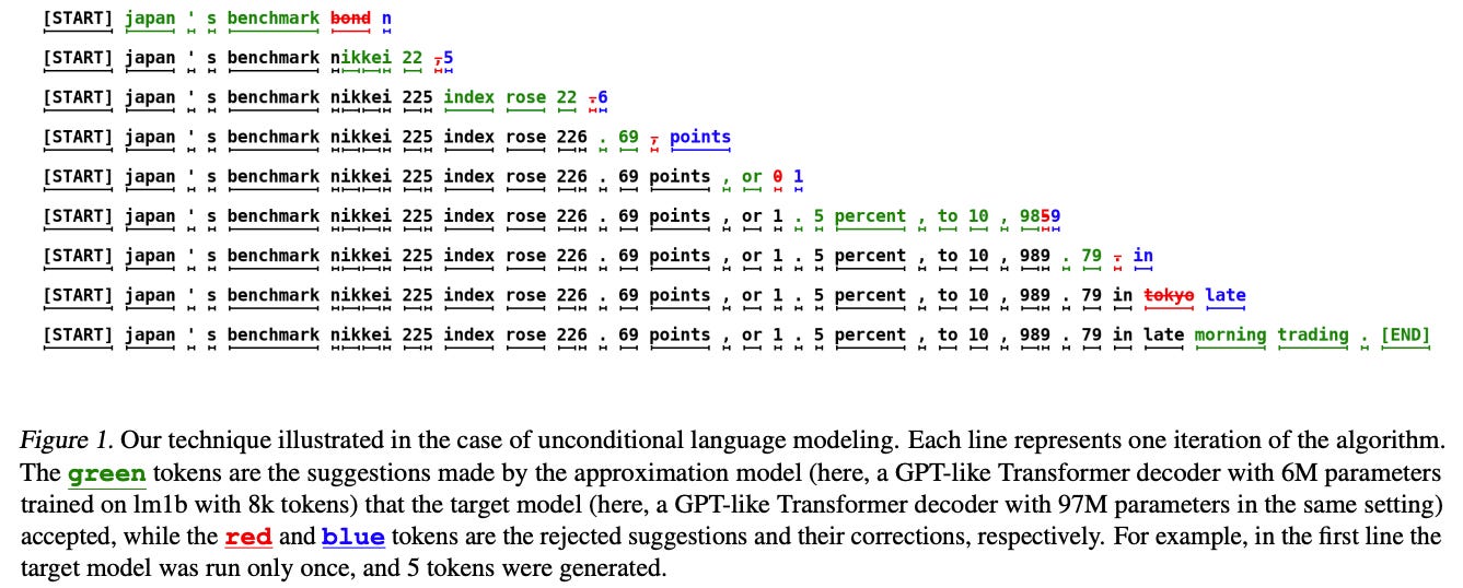
2. In the course of generation, most of the suggested tokens are accepted by the target model as evident in the image below.
What I liked:
Elegant fusion of fast and smart — utilizes existing models in a smart cooperative way.
Parallelism-friendly — large model verification can be done in parallel, increasing throughput.
No retraining required — works with any pre-trained small/large model pairs.
What I didn’t like:
Requires two models loaded simultaneously, so memory consumption still stays high.
Token acceptance/rejection adds a bit of control flow complexity, which might slow down edge-device deployments.
What could improve:
Learnable acceptance functions — instead of just thresholding based on logits, maybe train a tiny classifier to predict whether the large model would accept a token.
Entropy-informed sampling — dynamically decide how many draft tokens to generate based on entropy/confidence of small model predictions.
Applying it to vision models? Absolutely. Imagine a ViT-like encoder with a fast “draft” attention layer followed by a heavy “refiner” attention. Or multi-resolution vision inference, where low-res features guide high-res refinements — a speculative decoding analogue but for pixels.
This could also be seen from the perspective of a tracker model and a source model (as in object tracking), the tracker model works in intermediate step and source model jumps in picture as soon as the tracker pdf diverges to much from source pdf, now imagine tracker/draft model as a Kalman filter or a lower-order function and source/target model as higher-complexity model. Now this opens up a different way to think about everything we discussed till here.

A simple Kalman filter workflow, see how similar it is to everything that we discussed

Conclusion
In this blogpost we discussed about Speculative decoding and how it presents a clever trick — blend the speed of small models with the precision of big ones.
We started our discussion with issues around AR models as well as ideal way to solve it, then we talked about why speculative decoding promises a better solution? From there we delved into how speculative decoding works in great detail? then we saw simplest way to setup and use it. Finally we discussed the next steps and things I loved and possible improvements.
It's one of those "Why didn't we do this earlier?" ideas. A perfect example of engineering intuition meeting practical design.
With this we conclude our article for today.
For further nuances and details, please go through the paper here :
From Google : https://arxiv.org/pdf/2211.17192
From Deepmind : https://arxiv.org/pdf/2302.01318
That's all for today.
Follow me on LinkedIn and Substack for more insightful posts, till then happy Learning. Bye👋