
Transformers for Video: TimeSformer
TimeSformer brings Transformers to video by turning frames into patch tokens and using attention to model motion across time.

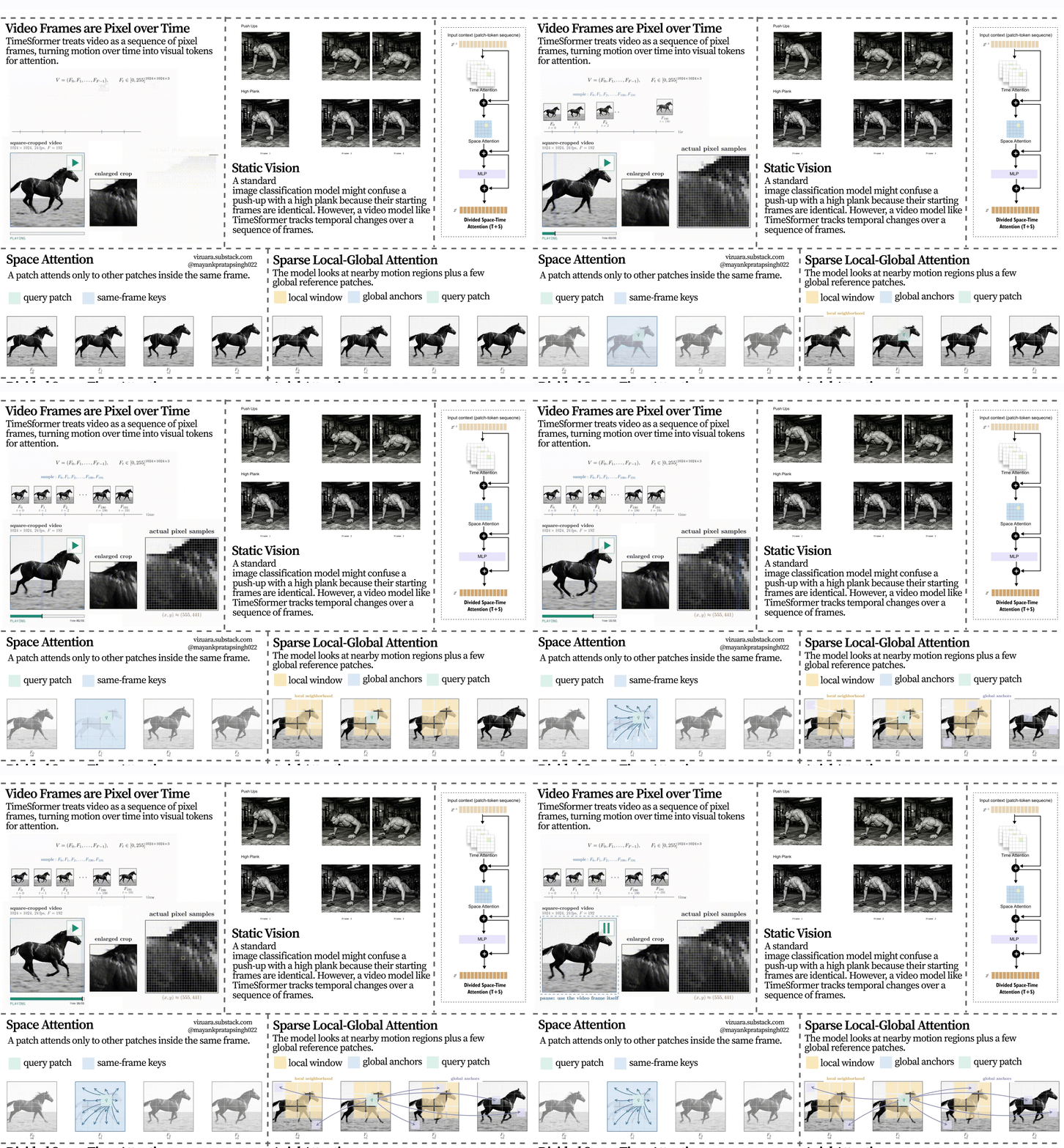
This chapter covers
Why video classification needs both spatial and temporal reasoning
How a video clip becomes a sequence of patch tokens
The self-attention equations used inside TimeSformer
Five space-time attention patterns: space-only, joint, divided, sparse local-global, and axial
Why divided space-time attention gives the best accuracy-efficiency tradeoff
How TimeSformer compares with 3D convolutional video models
How attention visualizations show what the model learns from video
Architectures like Vision Transformers and Convolutional Neural Networks treat an individual image as the core unit of visual understanding. Though analyzing them can be difficult, a single image remains a fixed grid of pixels. Video, however, adds the dimension of time; it is a sequence of images where meaning and labels heavily depend on observing how the scene evolves across frames.
TimeSformer, introduced by Bertasius, Wang, and Torresani in the ICML 2021 paper Is Space-Time Attention All You Need for Video Understanding?, asks a direct question: can we build a strong video recognition model using self-attention alone, without 3D convolutions? The answer from the paper is yes, provided that attention is arranged carefully over the space-time volume of a video clip.
The model starts from the Vision Transformer idea: split visual data into patches, embed those patches as tokens, add positional information, and feed the tokens to a transformer encoder. The difference is that a video has patches across both space and time. If every patch in every frame attends to every other patch, the computation becomes expensive very quickly. TimeSformer is mostly about how to make that attention usable.
Note
In this chapter, the word video means the visual stream only. TimeSformer, as presented in the paper, does not use the audio track. The task studied here is video classification: given a clip, predict one action label for the whole clip.
1.1 From images to videos
A still image classifier can sometimes solve a video task by looking at one frame. If the clip shows a cricket batter at the crease or a basketball player on the court, one frame may already contain enough context. But many action labels depend on motion. A frame from a push-up and a frame from a high plank can look nearly identical, while the sequence of frames makes the difference obvious.
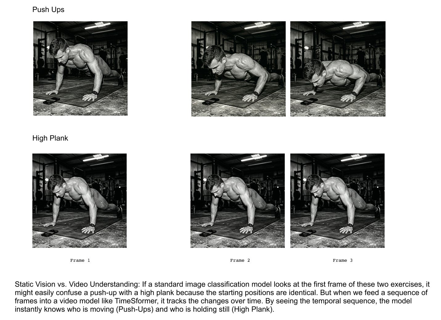
Figure 1.1. Static image classification can fail when two actions share nearly identical individual frames. In this example, a push-up and a high plank may look similar in a single snapshot. A video model must use the order of frames to detect whether the body is moving through an action or holding a static pose.
Figure 1.1 captures the central problem. A video model has to answer two questions at once: what is visible? and how is it changing? The first question is spatial. It concerns objects, body pose, background, and scene layout. The second is temporal. It concerns motion, ordering, repetition, and cause-effect patterns across frames.
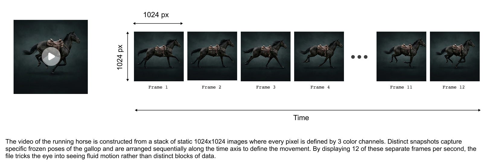
Figure 1.2. A video clip can be viewed as a sequence of images ordered along time. Each frame can be divided into patches, just as in a Vision Transformer, but the model now receives many grids of patches instead of one. The token sequence therefore grows with both image resolution and the number of frames.
The Kinetics datasets used in the TimeSformer paper contain short videos of human actions. They include labels such as headbanging, stretching a leg, shaking hands, tickling, robot dancing, and salsa dancing. Some labels are strongly tied to appearance; others require motion to disambiguate the action.
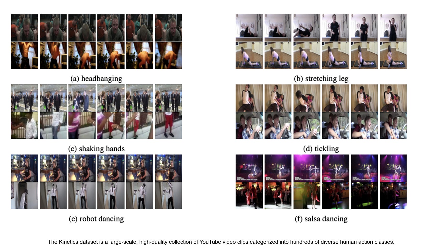
Figure 1.3. Examples from a Kinetics-style action recognition dataset. The model receives a short clip and predicts one action category for the whole clip. The examples show why both spatial context and temporal evidence matter: the person, object, and scene provide cues, but the action is often defined by movement across frames.
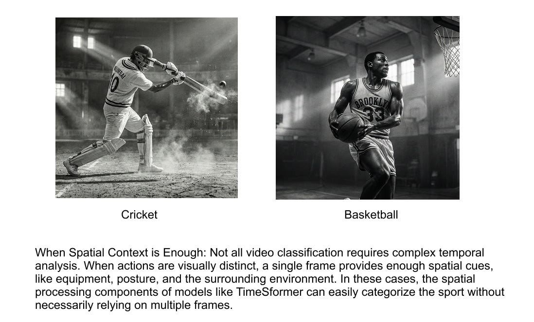
Figure 1.4. Some video labels can be predicted mostly from spatial context. A single frame of cricket or basketball already contains strong cues from the player, equipment, pose, and scene. TimeSformer still processes the clip as video, but examples like these explain why space-only attention can perform reasonably well on datasets with strong scene bias.
The opposite case is the reason TimeSformer is interesting. When appearance alone is ambiguous, the model needs to compare a region in one frame with related regions in later frames. This is where temporal attention enters.
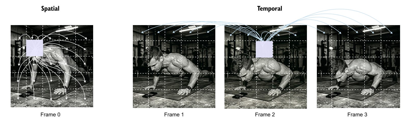
Figure 1.5. Spatial attention and temporal attention answer different questions. Spatial attention compares patches within a frame, such as the relationship between a hand, body, and background. Temporal attention compares corresponding or related patches across frames, allowing the model to represent motion and change over time.
1.2 Turning a video into tokens
TimeSformer follows the same tokenization idea as ViT, but applies it to every frame in a video clip. Let the input clip be
where F is the number of frames, H and W are the frame height and width, and the last dimension stores RGB channels. The TimeSformer paper writes the dimensions as H X W X 3 X F; both notations describe the same video volume.
Each frame is divided into non-overlapping patches of size P x P. The number of spatial patches per frame is
Across F frames, the clip contains NF patch tokens. A learned classification token is prepended, so the total token count is
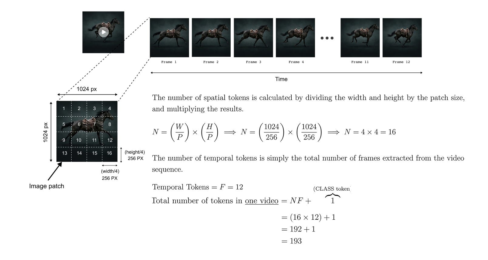
Figure 1.6. Counting the number of tokens in a video transformer. A frame is divided into spatial patches, and this patch grid is repeated for every sampled frame. The total sequence length is therefore the number of patches per frame multiplied by the number of frames, plus one class token for video-level classification.
The default TimeSformer setting in the paper uses clips of 8 x 224 x 224 and a patch size of 16 x 16 pixels. That gives
patches per frame and
tokens per clip. This is already much longer than the 197 tokens in a standard ViT image model with one 224 x 224 image and 16 x 16 patches.
For a patch at spatial index p and frame index t, the flattened RGB patch is
It is mapped to a D-dimensional embedding with a learned matrix E:
Here, epspace tells the model where the patch lies inside the frame, and ettime tells it which frame the patch came from. This separation is useful because a token has two coordinates: its spatial location and its temporal position.
1.3 Self-attention over a video
Once the clip is represented as tokens, TimeSformer uses the usual transformer ingredients: layer normalization, query-key-value projections, multi-head attention, residual connections, and an MLP. For head a in block l , query, key, and value vectors are computed as
The attention score between a query and a set of keys uses the same scaled dot-product rule as the original Transformer:
where dh = D / A is the feature dimension of one attention head. The output for a query token is the weighted sum of value vectors:
The set
is the important part. It defines which tokens a query is allowed to attend to. TimeSformer compares several choices for this neighborhood.
After attention, the heads are concatenated, projected, and passed through a residual MLP:
The final video representation is taken from the output class token:
A small classification head maps y to the video classes.
1.4 Five attention patterns
The TimeSformer paper studies five ways of arranging attention over space and time. The simplest way to understand them is to imagine choosing one query patch and asking: which other patches are allowed to become keys for this query?
1.4.1 Space-only attention
Space-only attention treats each frame almost like an independent image. A query patch attends to patches in the same frame, plus the class token:
This needs only N+1 key comparisons per query patch. It is cheap, and it can work when static appearance gives most of the answer. But it cannot directly model how a patch changes across frames.
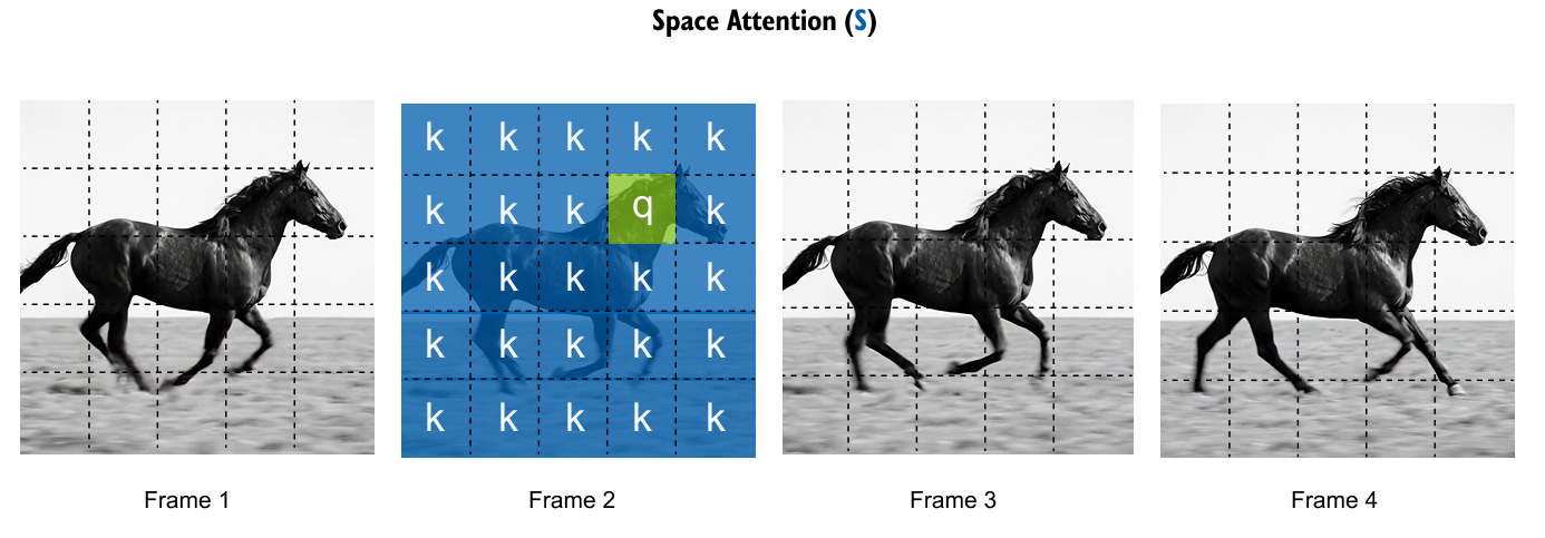
Figure 1.7. Space-only attention. The query patch attends to patches within the same frame, but it does not directly compare itself with patches in earlier or later frames. This pattern is efficient and can work for appearance-biased labels, but it discards explicit temporal reasoning.
1.4.2 Joint space-time attention
Joint space-time attention is the most direct extension of ViT to video. A query patch attends to every patch in every frame:
This gives the model full access to the video volume, but the cost grows quickly.
Each query compares against NF+1 keys, and the full attention matrix has size (NF+1) x (NF+1).
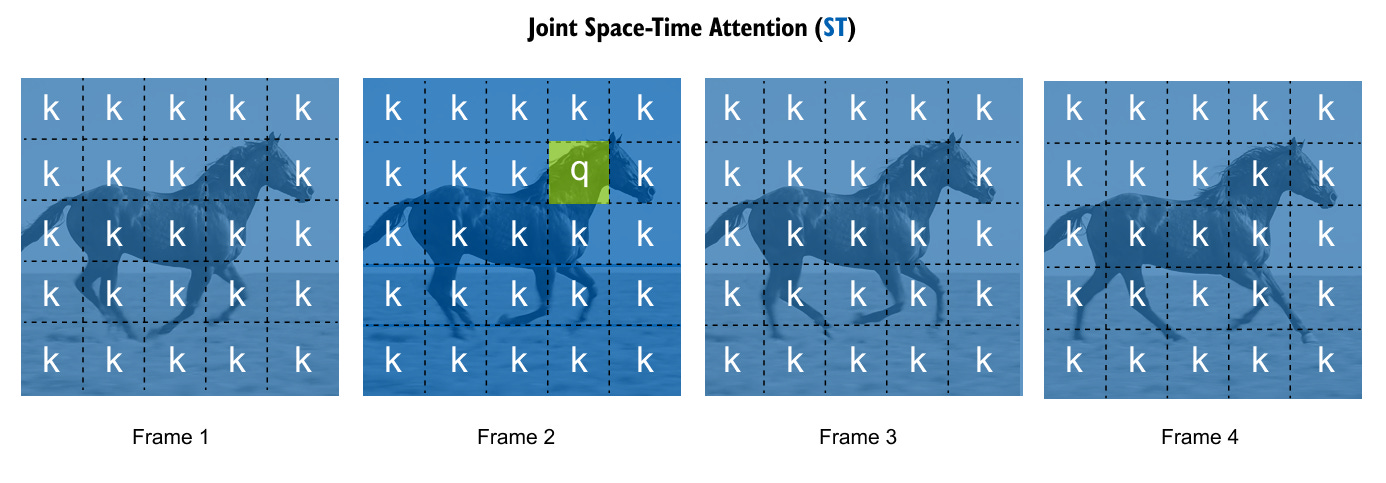
Figure 1.8. Joint space-time attention. The query patch can attend to all patches in all frames, giving the model a full global view of the clip. The drawback is computational cost: as resolution or video length increases, the number of pairwise comparisons becomes large enough to exhaust GPU memory.
For the default setting N=196 and F=8, joint attention gives each query 1569 possible keys. For a long clip with F=96, the same spatial resolution would give 18,817 keys per query. This is why a naive global video transformer is difficult to scale.
1.4.3 Divided space-time attention
Divided space-time attention is the main TimeSformer design. It factorizes the work into two smaller attentions inside each transformer block:
Temporal attention compares the same spatial patch location across frames.
Spatial attention compares patches within a frame.
For temporal attention, the neighborhood is
The output of temporal attention is fed into spatial attention, which then uses
In residual form, a divided TimeSformer block can be summarized as
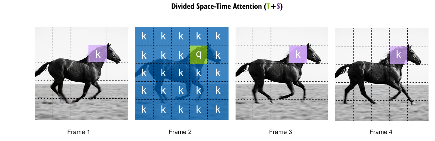
Figure 1.9. Divided space-time attention. The query first attends along the temporal axis at the same spatial patch location, then attends spatially within a frame. This gives the model access to both motion and appearance while avoiding the full quadratic cost of joint space-time attention.
Compared with NF+1 comparisons per query for joint attention, divided attention uses only
comparisons per query patch. With N=196 and F=8, this is 206 comparisons instead of 1569. With F=96, it is 294 instead of 18,817. The saving becomes larger as clips get longer.
1.4.4 Sparse local-global attention
Sparse local-global attention approximates full space-time attention by combining a local neighborhood with a sparse set of global locations. The local part captures nearby motion and appearance. The global part samples farther patches without attending to every possible location.
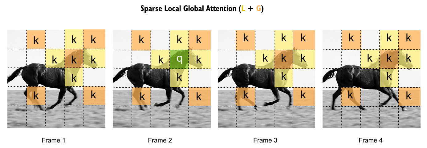
Figure 1.10. Sparse local-global attention. The query attends densely to a local space-time neighborhood and sparsely to farther locations. This gives the model some long-range context without paying the cost of full joint space-time attention. In the TimeSformer experiments, however, this pattern did not match divided attention’s accuracy.
1.4.5 Axial attention
Axial attention decomposes the video volume into one-dimensional passes. Instead of attending over the full space-time grid at once, it applies attention over time, then width, then height. This is another way to reduce cost by factorizing a high-dimensional attention problem.
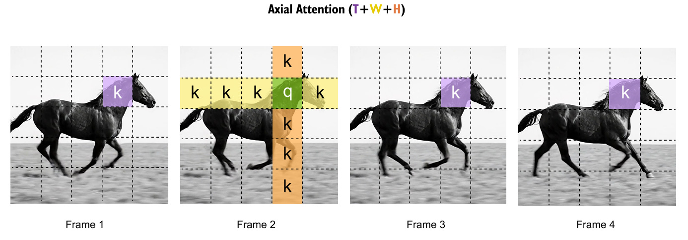
Figure 1.11. Axial attention. The model decomposes attention into separate passes along time, width, and height. This reduces the size of each attention operation, but it also imposes a stricter path for information flow through the video volume.
Figure 1.12 places the five attention blocks side by side. The diagrams also show where residual connections and MLP layers sit inside the block.
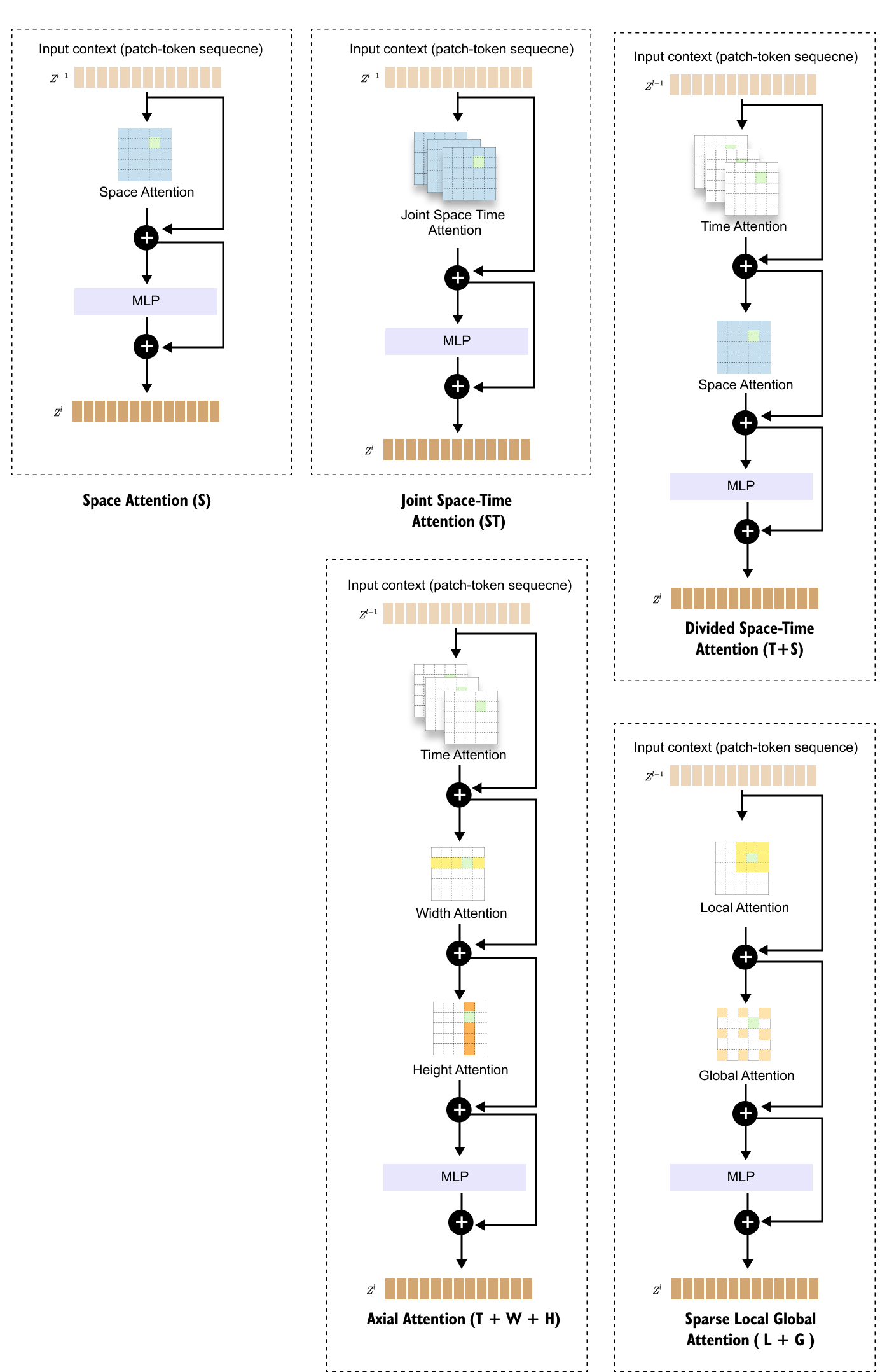
Figure 1.12. The five TimeSformer attention block designs compared in one view. Space-only uses one spatial attention layer, joint space-time uses one global attention layer, divided space-time uses temporal attention followed by spatial attention, sparse local-global combines local and sparse global passes, and axial attention applies attention along time, width, and height.
1.5 Why divided attention works well
At first, joint space-time attention sounds like the strongest option because it lets every token directly compare itself with every other token. The experiments tell a more practical story. Joint attention is expressive, but it is expensive, and it does not give the model separate parameters for temporal and spatial interactions. Divided attention uses separate temporal and spatial query-key-value projections, so it has more specialized capacity while still doing less pairwise work.
The cost difference becomes clear when the spatial crop or the number of frames increases.
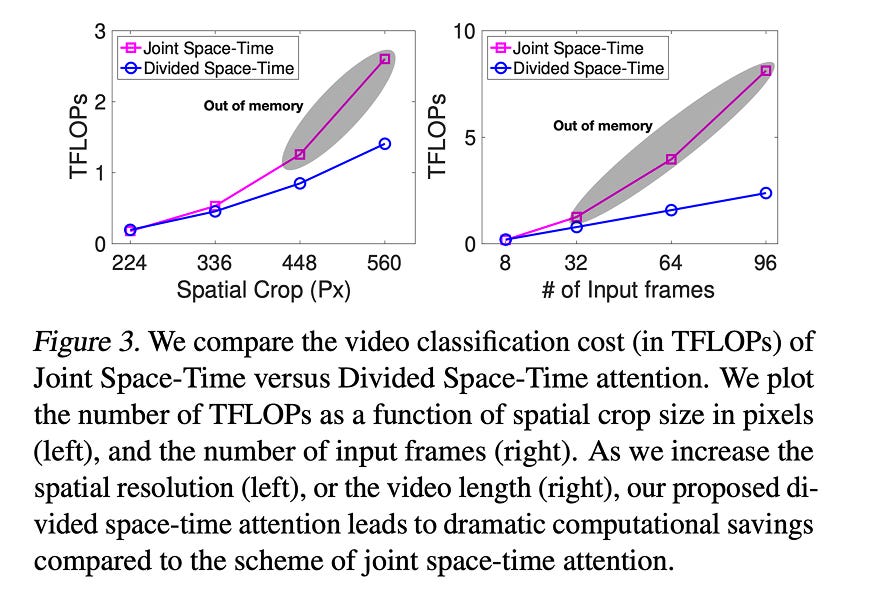
Figure 1.13. Computational cost comparison from the TimeSformer paper. Joint space-time attention becomes expensive as spatial crop size or input length grows, and it runs out of memory in the larger settings shown. Divided space-time attention scales more gently because it factorizes attention into temporal and spatial stages.
The accuracy comparison also favors divided attention.
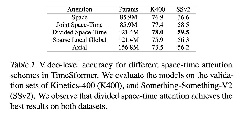
Figure 1.14. Video-level accuracy for the five attention schemes reported in the TimeSformer paper. Divided space-time attention obtains the best result on both Kinetics-400 and Something-Something-V2. Space-only attention performs well on Kinetics-400 but collapses on Something-Something-V2, which is a stronger test of temporal reasoning.
The table in Figure 1.14 is worth reading carefully. Space-only attention reaches 76.9% on Kinetics-400, which confirms that many Kinetics labels can be predicted from appearance. But it reaches only 36.6% on Something-Something-V2. That dataset contains labels where the same objects can appear in different actions, so temporal order matters much more. Divided attention reaches 78.0% on Kinetics-400 and 59.5% on Something-Something-V2, beating the other attention patterns in the paper’s comparison.
Note
The main lesson is not that temporal attention should replace spatial attention. The lesson is that video classification needs both, but not necessarily in one huge attention matrix. TimeSformer gets a strong result by making time and space separate operations inside the same block.
1.6 An implementation view
The implementation idea behind divided attention is simple once the tensor shape is clear. Suppose the token tensor, after removing or separately handling the class token, has shape
where B is the batch size. Temporal attention should see F as the sequence dimension while keeping a fixed spatial patch index. Spatial attention should see N as the sequence dimension while keeping a fixed frame.
Listing 1.1.
The tensor reshaping pattern behind divided space-time attention. Temporal attention groups batch and spatial patch index together, so attention runs across frames. Spatial attention groups batch and frame index together, so attention runs across patches inside one frame.
# x has shape [B, F, N, D]

# Temporal attention: sequence length is F.
x_t = rearrange(x, "b f n d -> (b n) f d")
x_t = temporal_attention(x_t, x_t, x_t)
x = rearrange(x_t, "(b n) f d -> b f n d", n=N)

# Spatial attention: sequence length is N.
x_s = rearrange(x, "b f n d -> (b f) n d")
x_s = spatial_attention(x_s, x_s, x_s)
x = rearrange(x_s, "(b f) n d -> b f n d", f=F)
Listing 1.1 is not a full TimeSformer implementation, but it captures the core trick. To apply temporal attention, we flatten the batch and patch dimensions into one larger batch and let the attention module process the frame dimension. To apply spatial attention, we flatten the batch and time dimensions and let the attention module process the patch dimension.
The full model also needs patch embedding, a class token, space and time positional embeddings, layer normalization, MLP blocks, and a classification head. These are inherited from the transformer and ViT design. TimeSformer’s main change is how attention is scheduled over a video.
1.7 What the model learns
Attention visualizations help make the model less abstract. When TimeSformer predicts a Something-Something-V2 action, the attended regions often track the object or the hand-object interaction that defines the action.
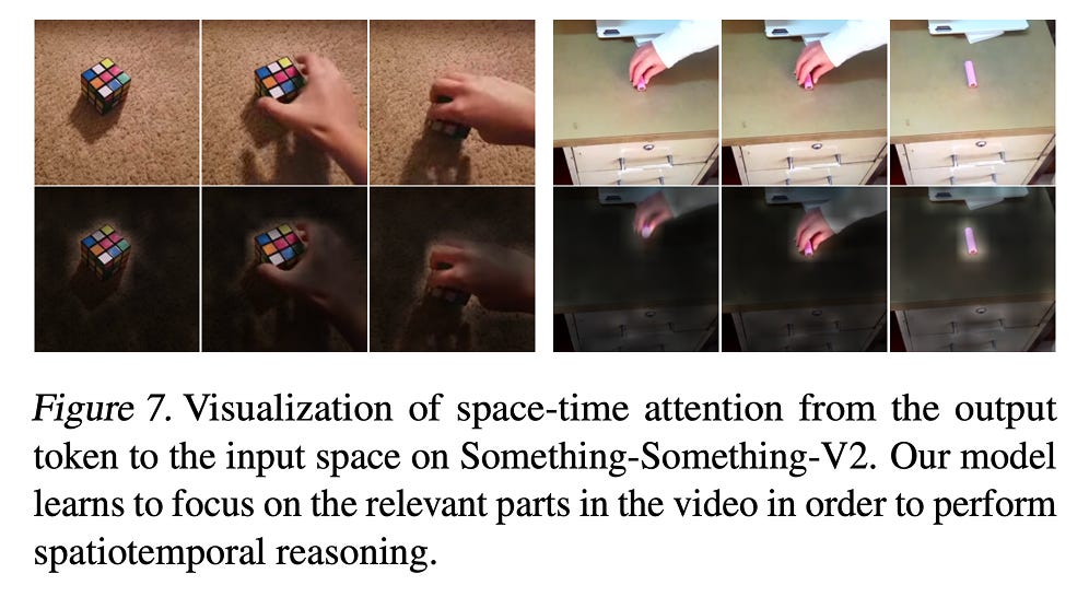
Figure 1.15. Space-time attention visualization from the TimeSformer paper. The highlighted regions show that the model focuses on task-relevant areas, such as the hand and manipulated object, rather than spreading attention uniformly over the frame. This is the behavior expected from a model that must reason about actions, not just objects.
The paper also visualizes learned video embeddings with t-SNE. Each point represents a video, and videos with the same action label share a color. The divided-attention model forms more separable clusters than ViT or a space-only TimeSformer.
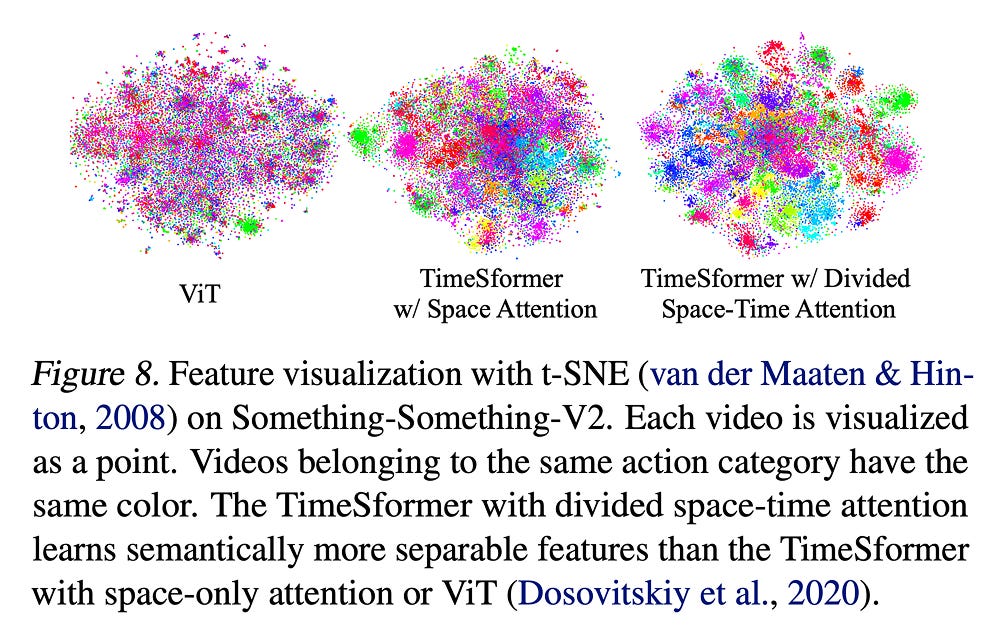
Figure 1.16. Feature visualization from the TimeSformer paper. The divided space-time model forms more separated action clusters than a space-only model or a ViT baseline. This suggests that the temporal branch is not merely adding computation; it changes the learned representation in a way that separates actions more cleanly.
These visualizations do not prove causal reasoning by themselves, but they support the quantitative result: modeling time explicitly improves the representation for action recognition.
1.8 Comparison with 3D convolutional models
Before video transformers, strong video classifiers were usually built from 3D convolutions. A 3D convolution slides a local kernel over height, width, and time. This gives the model a built-in local motion bias, which is useful, but it also means long-range relationships must be built gradually through many layers.
TimeSformer takes a different route. Self-attention can connect distant patches directly, and divided attention keeps the cost manageable enough to process longer clips. The paper reports that the default TimeSformer has 121.4 million parameters but only 0.59 TFLOPs of inference cost for the reported setting, compared with 1.97 TFLOPs for a SlowFast R50 model in the same comparison.
The larger TimeSformer-L variant processes 96 input frames and reaches 80.7% top-1 accuracy on Kinetics-400 in the paper’s reported table.
The official TimeSformer repository provides pretrained model variants for Kinetics-400, Kinetics-600, Something-Something-V2, and HowTo100M, including longer-input models that cover much more temporal context than the default 8-frame setting. The Hugging Face Transformers documentation also exposes TimeSformer as a video classification model, which makes the architecture easier to reuse in modern transformer workflows.
The practical tradeoff is clear. TimeSformer benefits from image pretraining and large datasets, while 3D CNNs still offer strong inductive biases and can be easier to train in smaller-data settings. But the paper showed that a convolution-free video model was no longer just a curiosity. With the right attention pattern, transformers could compete seriously on video recognition.
1.9 Resources
- Video:
In this video, Dr. Sreedath Panat. explains how to implement TimeSformer from scratch and walks through the main building
blocks of the model.
- Paper:
Is Space-Time Attention All You Need for Video Understanding?
Summary
A video clip can be represented as a sequence of frame-level patches. If each frame has N patches and the clip has F frames, the transformer receives NF+1 tokens, including the class token.
Space-only attention compares patches within the same frame. It is efficient and can work on appearance-biased datasets, but it cannot explicitly model motion across frames.
Joint space-time attention compares every patch with every patch in every frame. It is expressive, but its cost grows quickly with spatial resolution and clip length.
Divided space-time attention factorizes the work into temporal attention followed by spatial attention. This reduces the comparisons per query from NF+1 to N+F+2 while still modeling both motion and appearance.
In the TimeSformer paper’s comparison, divided space-time attention achieves the best accuracy among the five studied schemes on both Kinetics-400 and Something-Something-V2.
TimeSformer differs from 3D CNNs by replacing local convolutional kernels with attention over patch tokens. This gives it a direct route to long-range video modeling, especially when enough data and pretraining are available.
Attention and feature visualizations show that the divided model learns representations that focus on action-relevant regions and separate video classes more clearly than space-only variants.
More Blogs


I’m also building Audio Deep Learning projects and LLM projects, sharing and discussing them on LinkedIn and Twitter. If you’re someone curious about these topics, I’d love to connect with you all!
Mayank Pratap Singh
LinkedIn : www.linkedin.com/in/mayankpratapsingh022
Twitter/X : x.com/Mayank_022.