
Understanding RLHF From Scratch
A beginner's guide to understanding RLHF from Scratch

Let us start by understanding how Reinforcement Learning is applied to language models.
Let us take a simple example:
If we ask the following question to a language model:
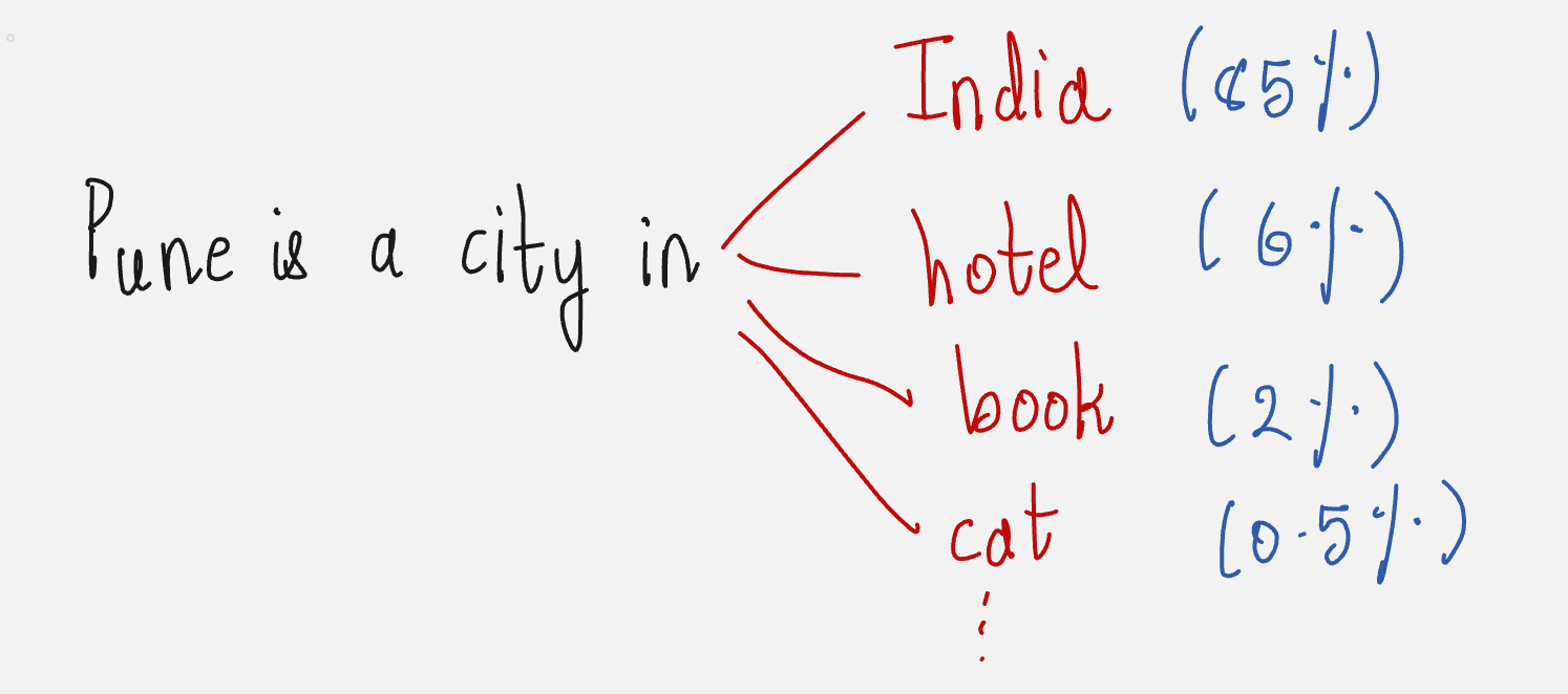
Pune is a city in ___
The language model will probably give an answer which looks something like this:
Pune is a city in India.
We get the correct answer because the language model is trained to predict the token which has the highest probability as the next token.
Integrating Reinforcement Learning in LLMs:
So far, we have learned about Reinforcement applied in general settings.
Now we will begin to understand how Reinforcement Learning can be used to improve language models.
We first need to understand what are the states, actions, and rewards.
Let us take an example:
I am going ___
What is the next word?
The next word depends on the previous set of words.
So here, the state is the combination of the three previous words.
The action is the next word in the sequence.
The reward denotes the “coherency” of the action given the input state. We will look at how to quantify this coherency later.
What about the policy?
The policy is the probability of taking an action for the current state of the agent.
For large language models, the policy is the probability of predicting the “next token” given the “current tokens”.
This is the LLM itself.

In other words, in a large language model, the agent is the same as the policy, which is the LLM itself.
This might sound a bit weird, but it is true.
Notations:
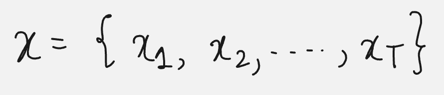
Prompt(x): The input text given to a language model to generate a response.
The prompt is made up of a sequence of tokens.
The token is a basic unit for text. It can be a word or a single character.

So, the prompt is made up of a sequence of tokens.
Completion (y): The output text generated by a model in response to a prompt. The completion is often denoted as y|x.
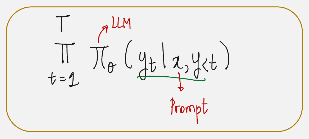
Policy: Modern language models learn how likely a sentence is by predicting one word at a time based on all the words that came before it.
For example, consider the sentence: “I like to eat pizza”
The model will do this :
(1) Predict “I”
(2) Predict “like” - given “I”
(3) Predict “to” - given “I like”
(4) Predict “eat” - given “I like to”
(5) Predict “pizza” - given “I like to eat”
So, the probability of the whole sentence is given by:
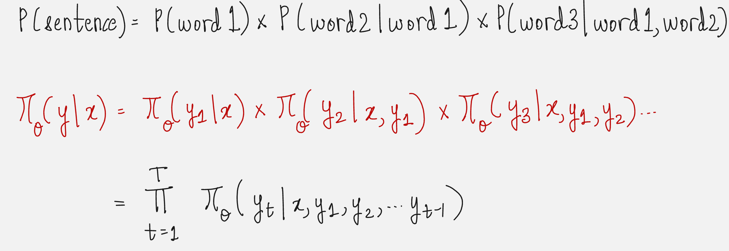
This is also represented as:
Okay, enough mathematics!
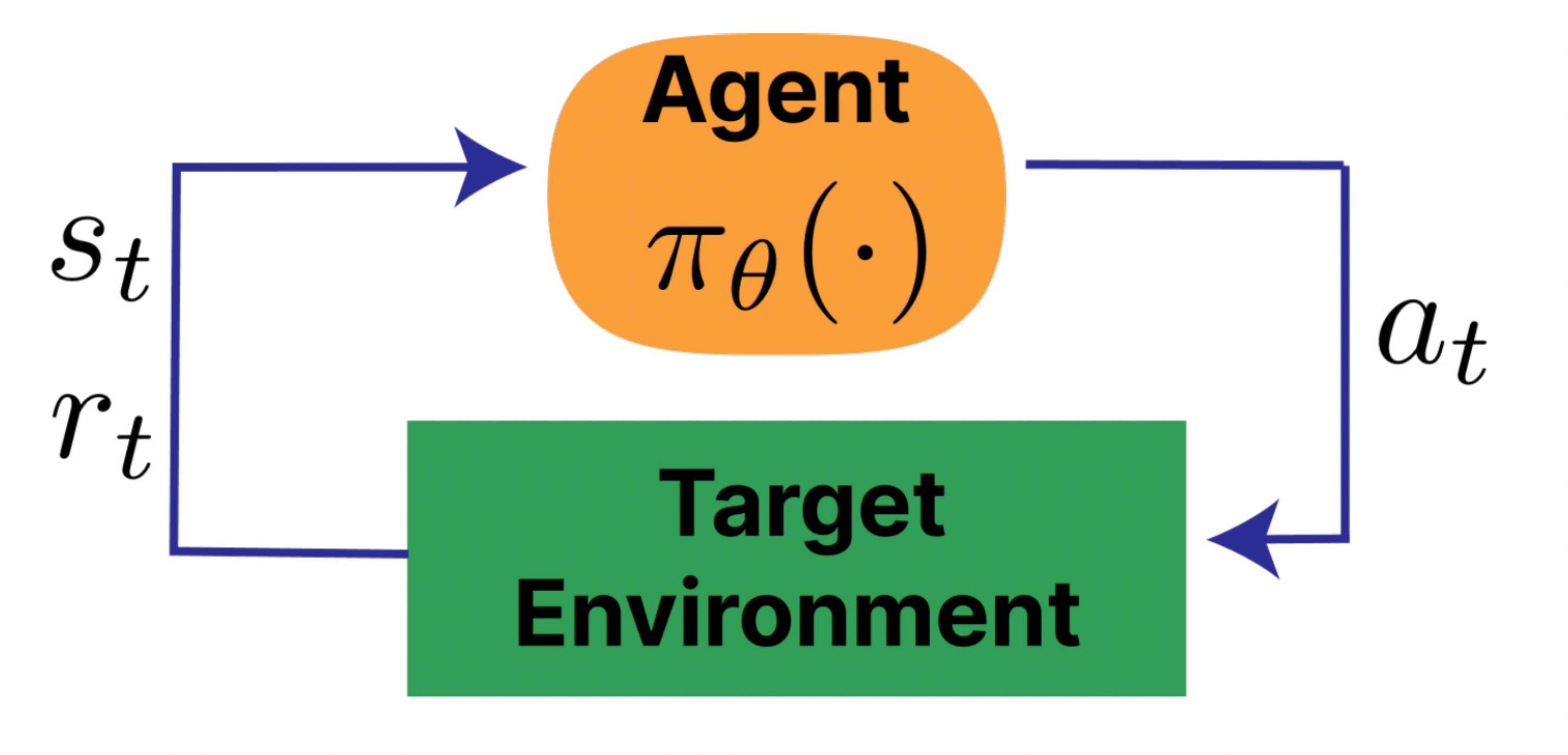
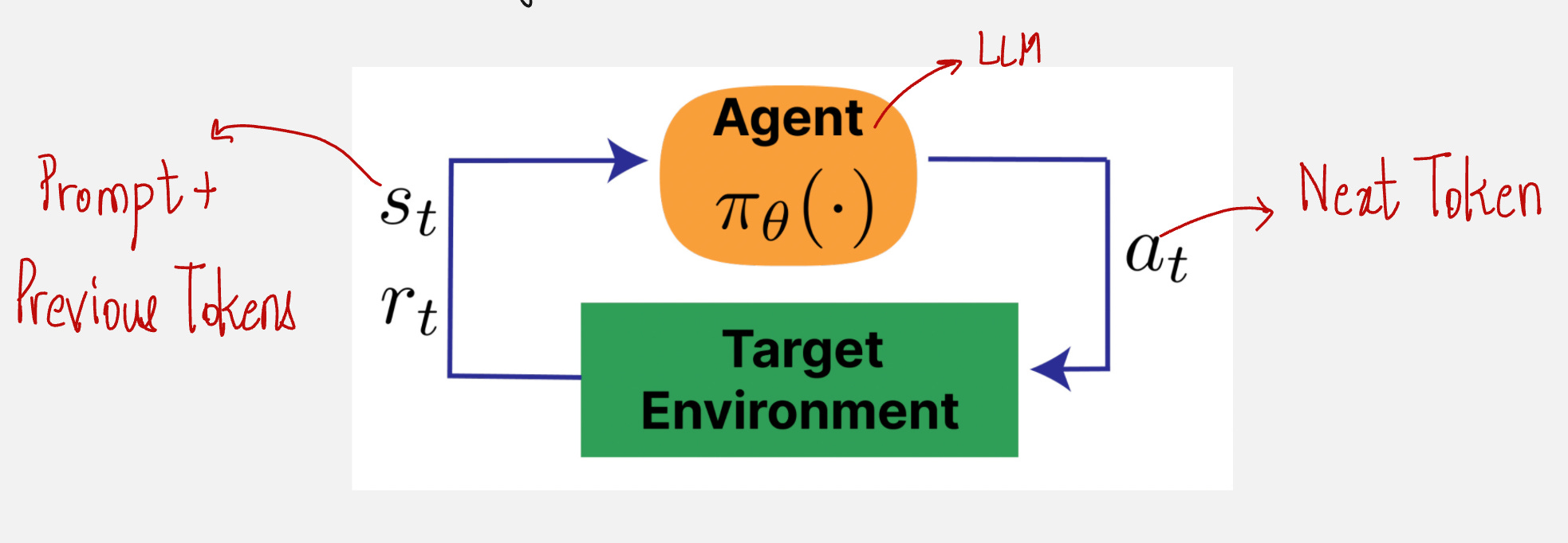
We can draw the agent-environment interface for language models as follows:
Okay, but what about the rewards?
Reward Modeling:
For objective questions, it is easy to assign rewards because we can judge the answers easily.
For example:
Prompt: What is 2+2?
Answer: 4
Reward: High (easy to verify)
But for subjective questions, humans are not good at finding a common ground for agreement.
For example:
Prompt: Explain RLHF like I am a 5 year old
Answer: RLHF is used for aligning models
Reward: Subjective (Not easy to verify)
But we are good at comparing.
Assigning Rewards by Comparison:
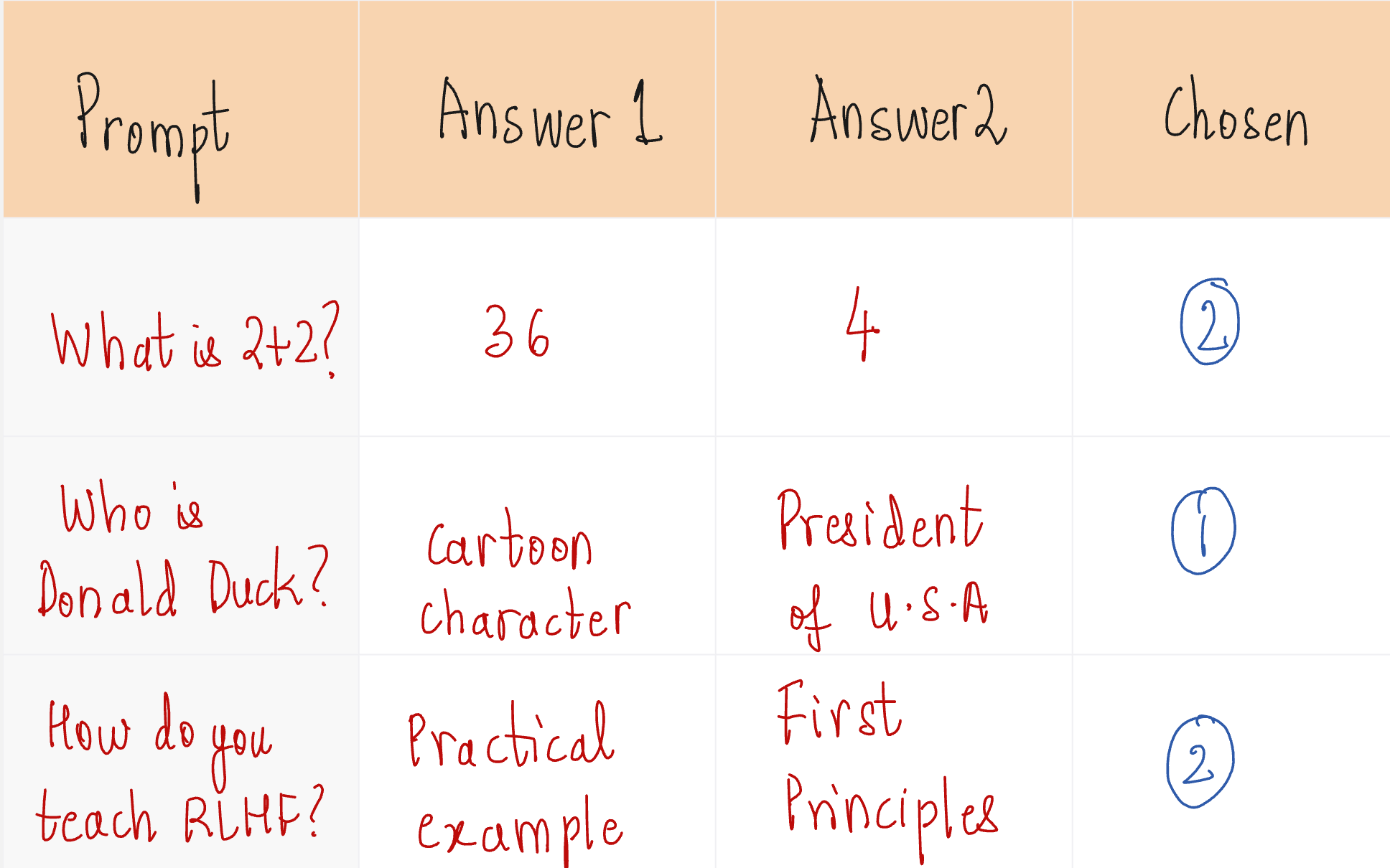
You can see from the above examples that giving preferences comes naturally to us.
Okay, but how do we actually calculate the rewards?
For this, we use something called the Reward Model.
Reward Model Building:
The reward model is built from the LLM architecture itself with two main differences:
(1) The hidden states are not projected into the vocabulary.
(2) Only the final hidden state is passed as an input to a linear layer to get a single scalar value as the reward.
The reward model architecture looks as follows:
To train our reward model, we need to define the loss function.
Let us look at an example to understand how this loss function is defined.
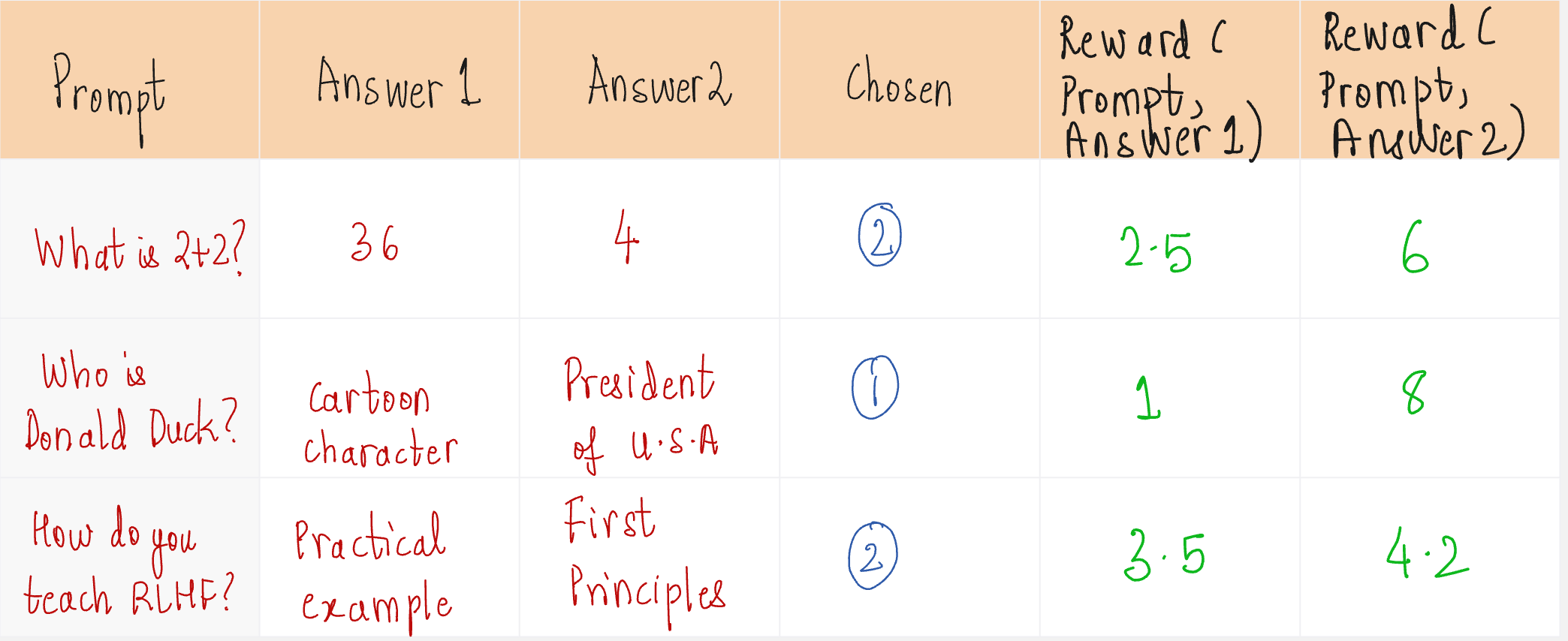
In the above example, except for the second case, our model assigns higher rewards for preferred answers, which is what we want.
If the preferred response is denoted by y_w and the rejected response is denoted by y_l, and the prompt is denoted as x,
The loss is defined by the following function:
Let us understand this by taking two cases:
Case 1:
This means that our model is assigning a higher reward to the chosen response compared to the rejected response, which is exactly what we want.
So the loss should be low.
Let us see if that is really the case:
The sigmoid function looks as follows:
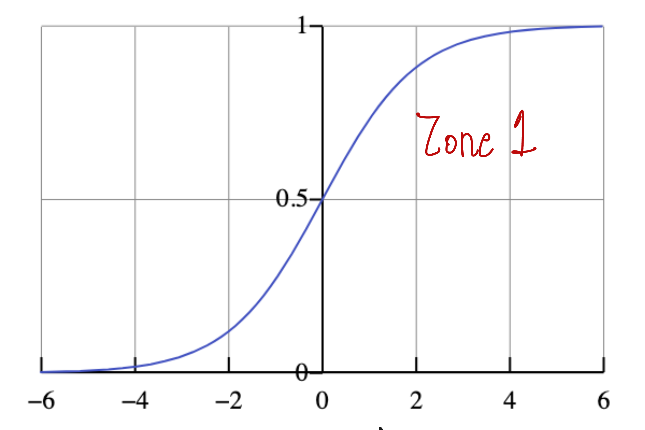
And the loss function by taking the log of the sigmoid function looks as follows:
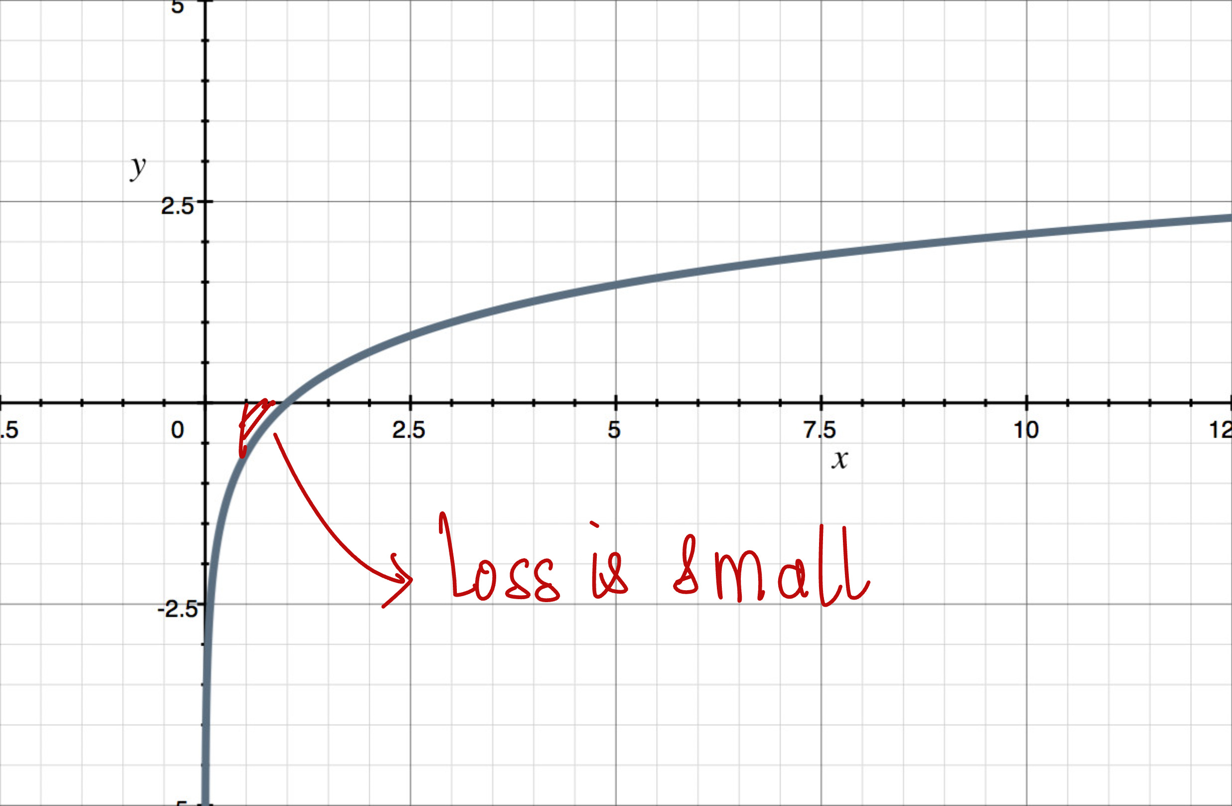
The loss is small, which is what we wanted.
Now let us check for the second case.
Case 2:
This means that our model is assigning higher rewards to the rejected response compared to the chosen response.
This is not what we want.
So the loss should be higher in this case.
Let us see the sigmoid and the log function.
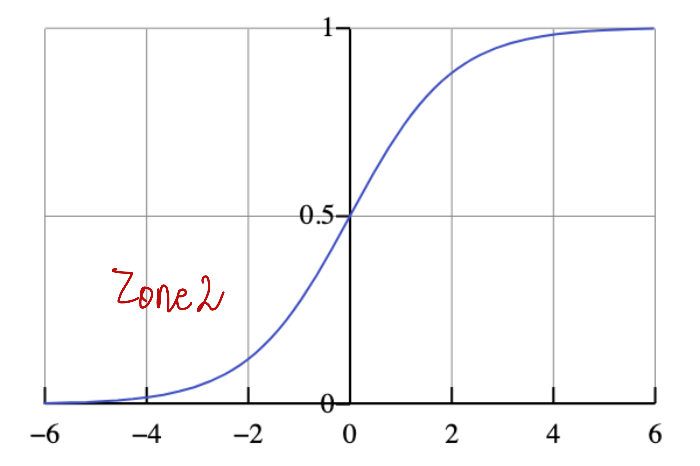
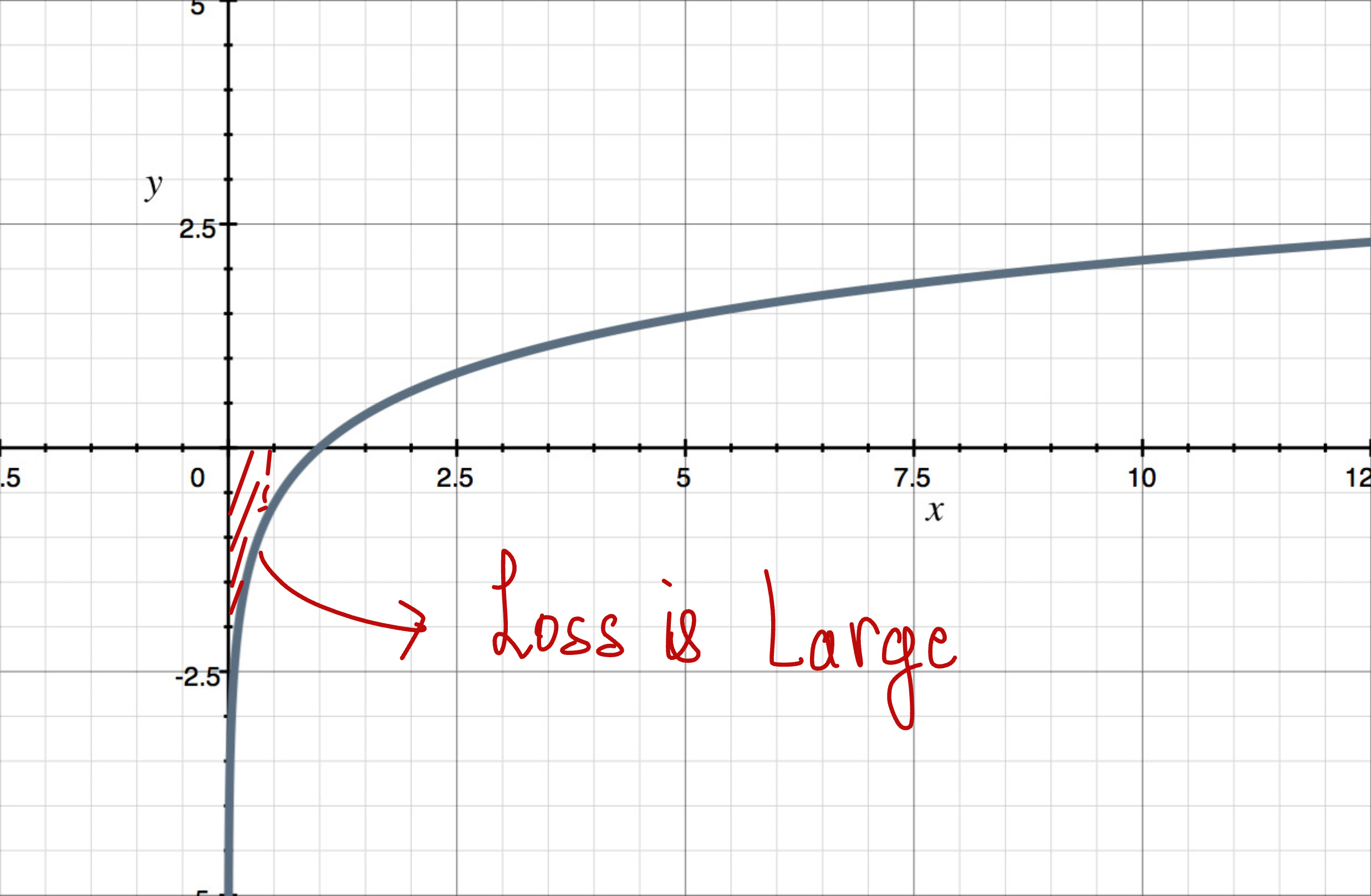
The loss is very high, which is exactly what we want.
So, the loss function that we have defined works fine.
To understand how LLMs are improved using reinforcement learning, it is very important for us to first understand about policy gradients.
I have written a separate article which explains about the policy ingredients completely from scratch. You can find the article here: Policy Gradient from Scratch
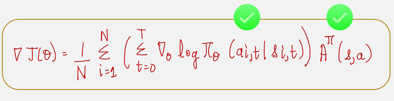
From our previous lecture on Policy Gradients, we know that the gradient of the performance measure is given by the following formula:
I know this looks a little complicated, but essentially what we are doing is:
Calculating the log probabilities for all the actions in a given trajectory
Multiplying it by the advantage
Taking an average over for all the possible trajectories
Let us understand what each of the terms in the above expression means for a language model.
Let us take an example.
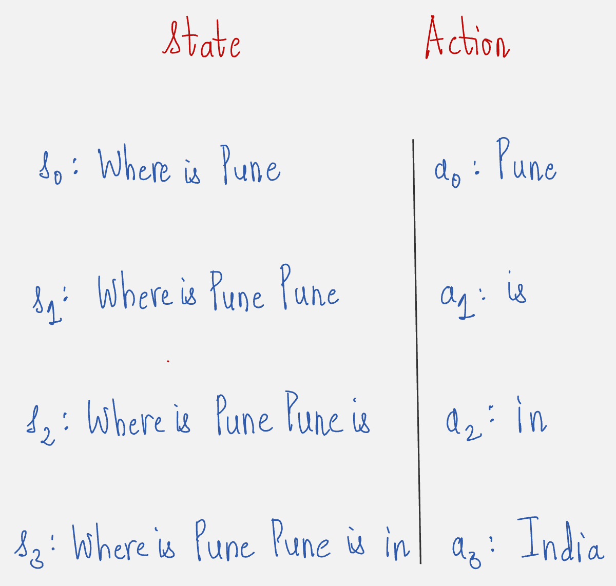
Prompt: Where is Pune
Answer: Pune is in India
First, let us map this to a trajectory of states and actions:
Now we will understand how the log probabilities of the actions are calculated.
Have a look at the schematic below:
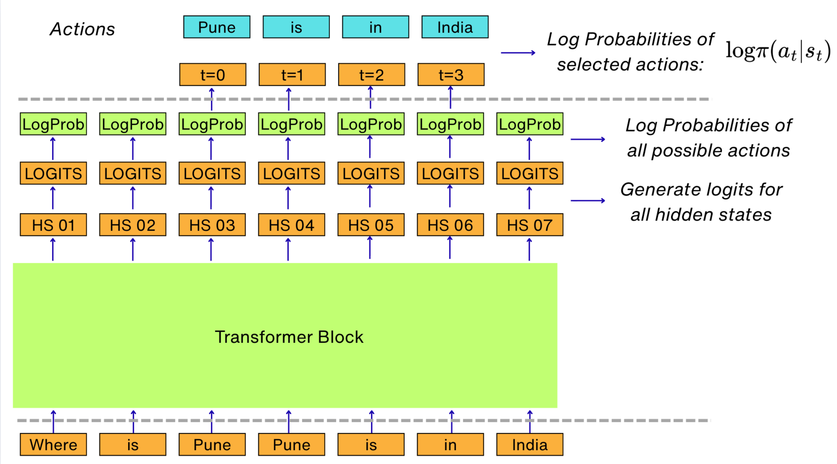
The way our architecture of the LLM works, the log probabilities of all the possible actions can be calculated directly from the logits generated from the hidden states. After that, we only select the log probabilities of the actions which are selected.
For example, in our example, we have four selected actions: “Pune”, “is”, “in” and “India”. So, we calculate the log probabilities for these actions.
So, we have taken care of the following part of the gradient of the performance measure:
What about the advantage function?
To calculate the advantage function, a method called Generalized Advantage Estimation is used. From this method, we know that the advantage function can be solely estimated from the value function.
You can refer to my notes on Generalized Advantage Estimation here: Notes on Generalized Advantage Estimation
So the next question is: How do we estimate the value function?
The value function is exactly the same as LLM.
The only difference being that the logits are not projected into the vocabulary space.
Instead, the logits are transformed using a single linear layer to a single value.
Have a look at the schematic below:
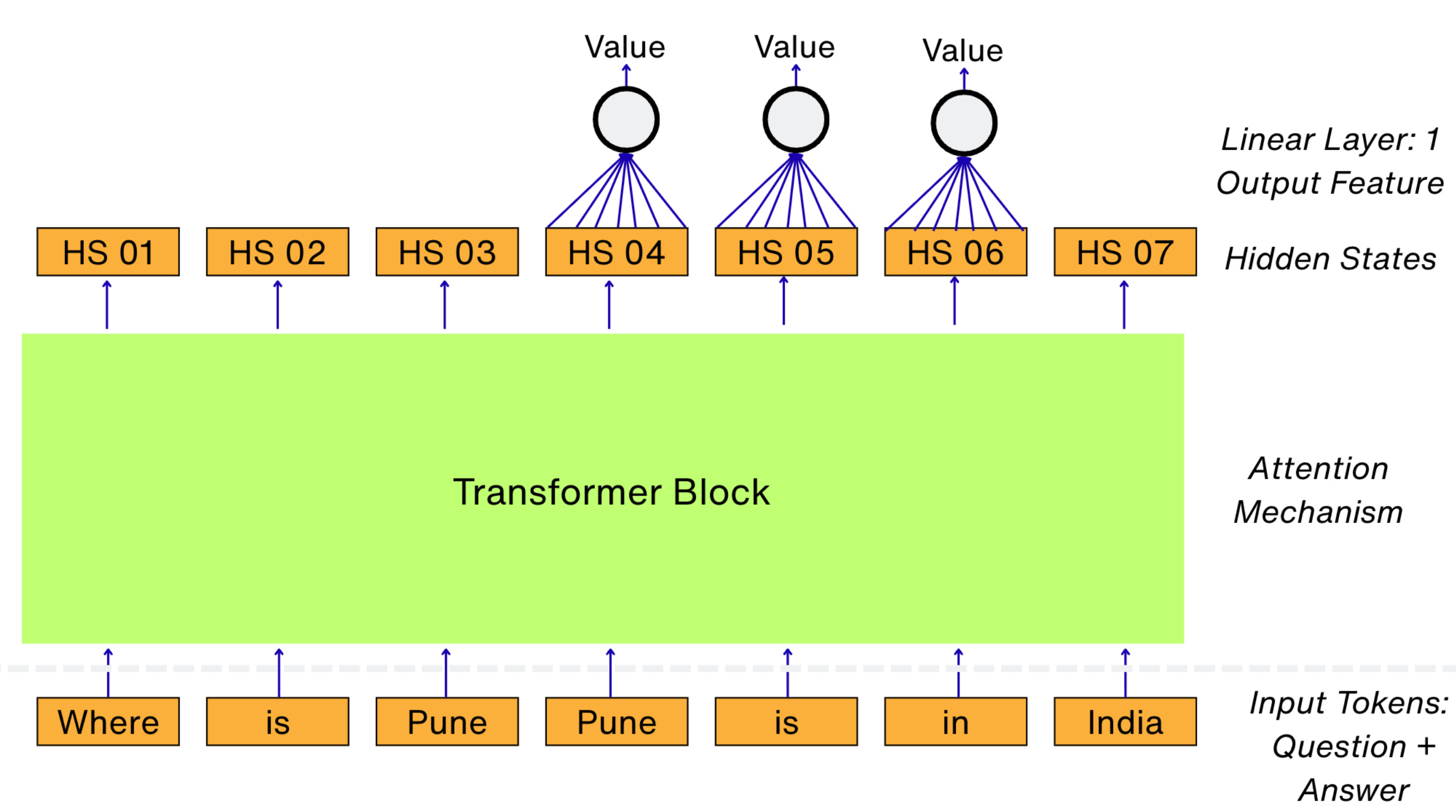
Using the value function estimate, we can now evaluate the advantage function.
Now let us look at our expression for the gradient of the performance measure:
Looks like we're all set now.
Almost…
We have one last step to understand.
Reward Hacking
Let us say our reward model is trained to give positive rewards to happy sentiments and negative rewards to sad sentiments.
During the RL training, our LLM might “hack” the reward.
This means that our LLM might figure out that using happy, love, or thank you is giving more rewards.
It can then start using more and more positive words without caring about the context.
We need to prevent this from happening. We need to prevent our model from deviating too far from our reference model which already works decently.
This is done by measuring how much is the difference in the log probabilities of the same token predicted by our language model and the frozen model.
An objective metric of measuring the difference between two probability distributions is the KL Divergence.
The schematic below explains how the KL Divergence is calculated for the predicted tokens for a given prompt.
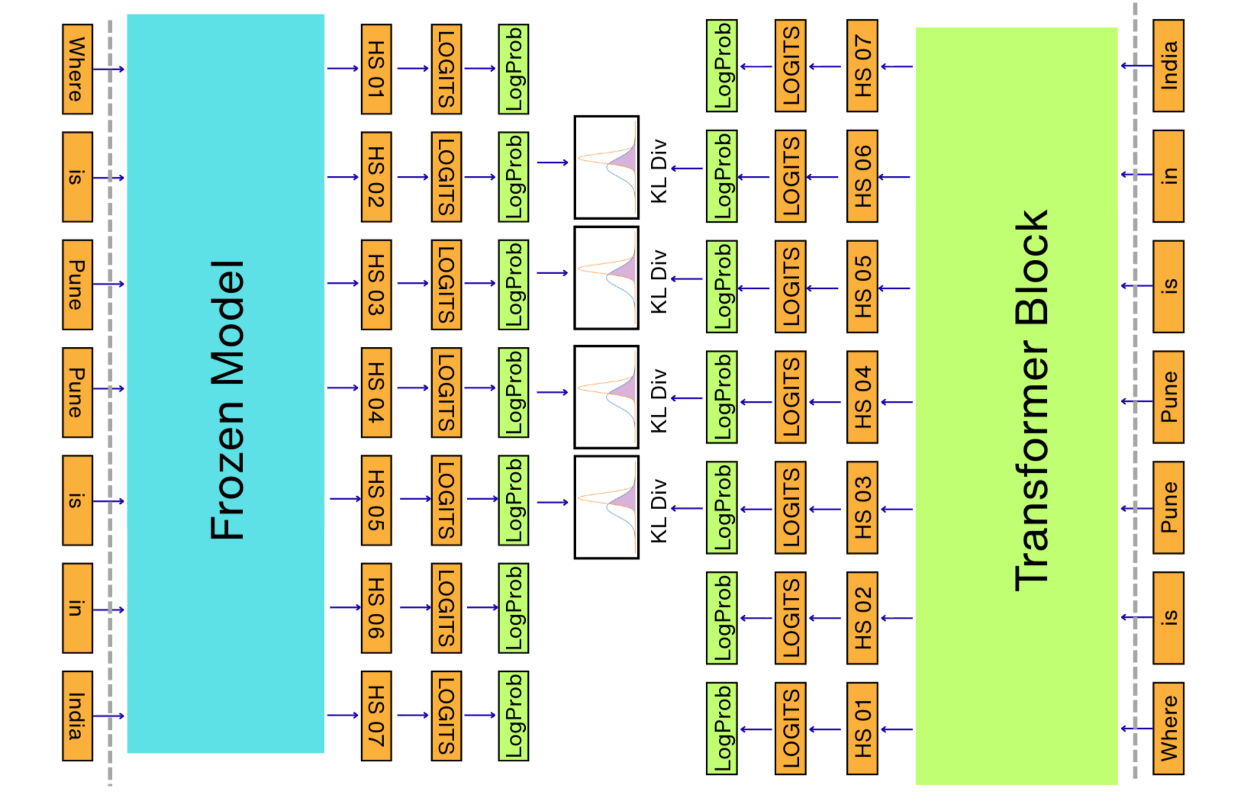
You might have to rotate your screen to look at this diagram, but if you look closely, you will understand that the KL divergence is calculated from our current LLM that we are trying to optimize and the reference LLM which is the frozen model.
The reward for each state-action pair is then calculated as follows:
Let us now look at an example where all this knowledge is applied to a practical example.
Entire RLHF pipeline to fine-tune GPT-2 micro to align output towards positive sentiments.
(1) Our model :
We are using a tiny model (GPT-2 micro)
4 layers, 3 heads per layer, model dimensions: 128 (~1M parameters)
(2) Our dataset:

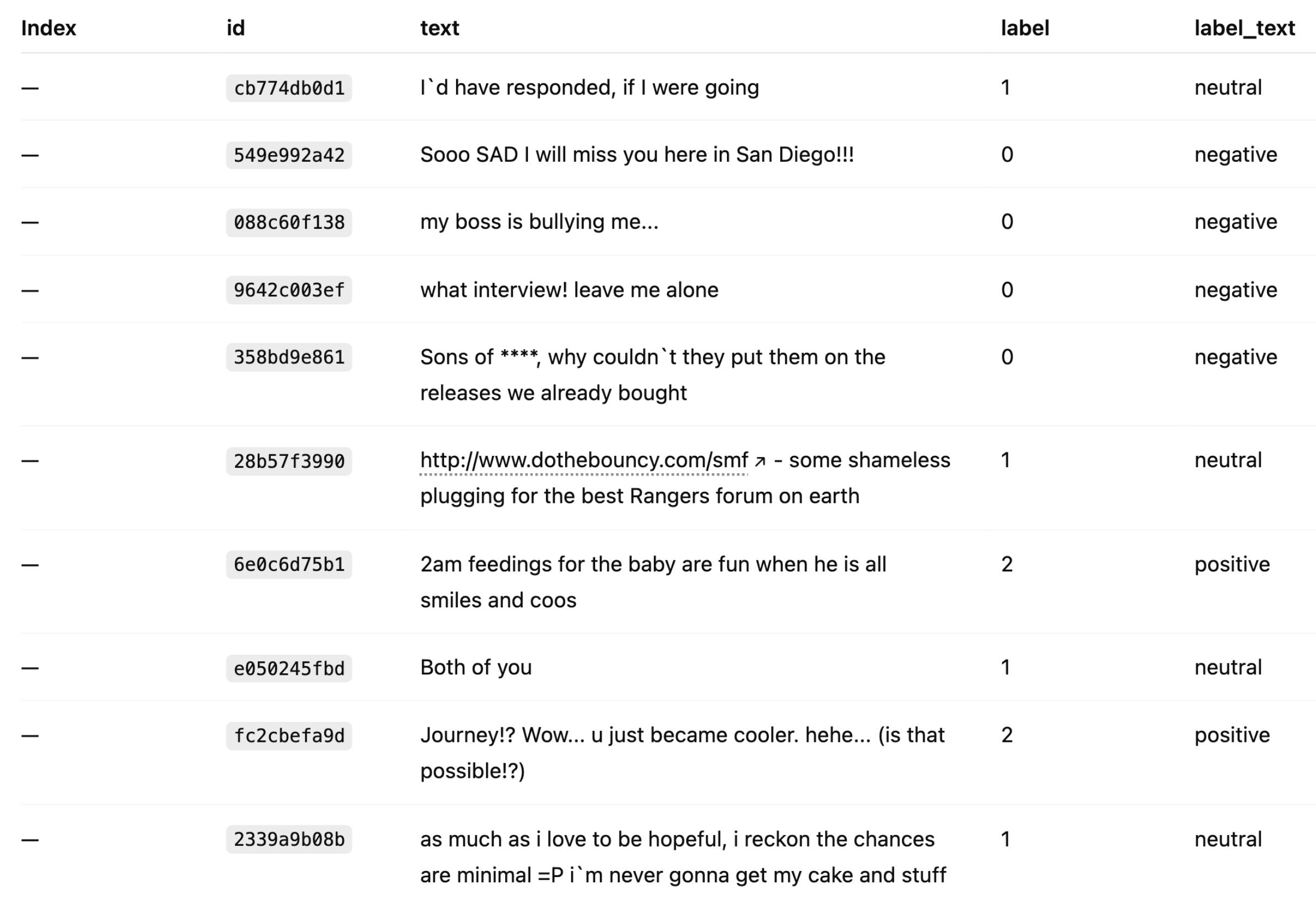
We will be training our model on 50,000 tweets.
(3) Methodology:
We will be implementing the following steps for analysis:
Pre-training
Supervised fine-tuning
Reinforcement training with verifiable rewards
We will use the policy gradient method for this approach.
In this article, we will focus on the Reinforcement Learning step.
The overall flow for the Reinforcement Learning step using Vanilla Policy Gradient looks as follows:
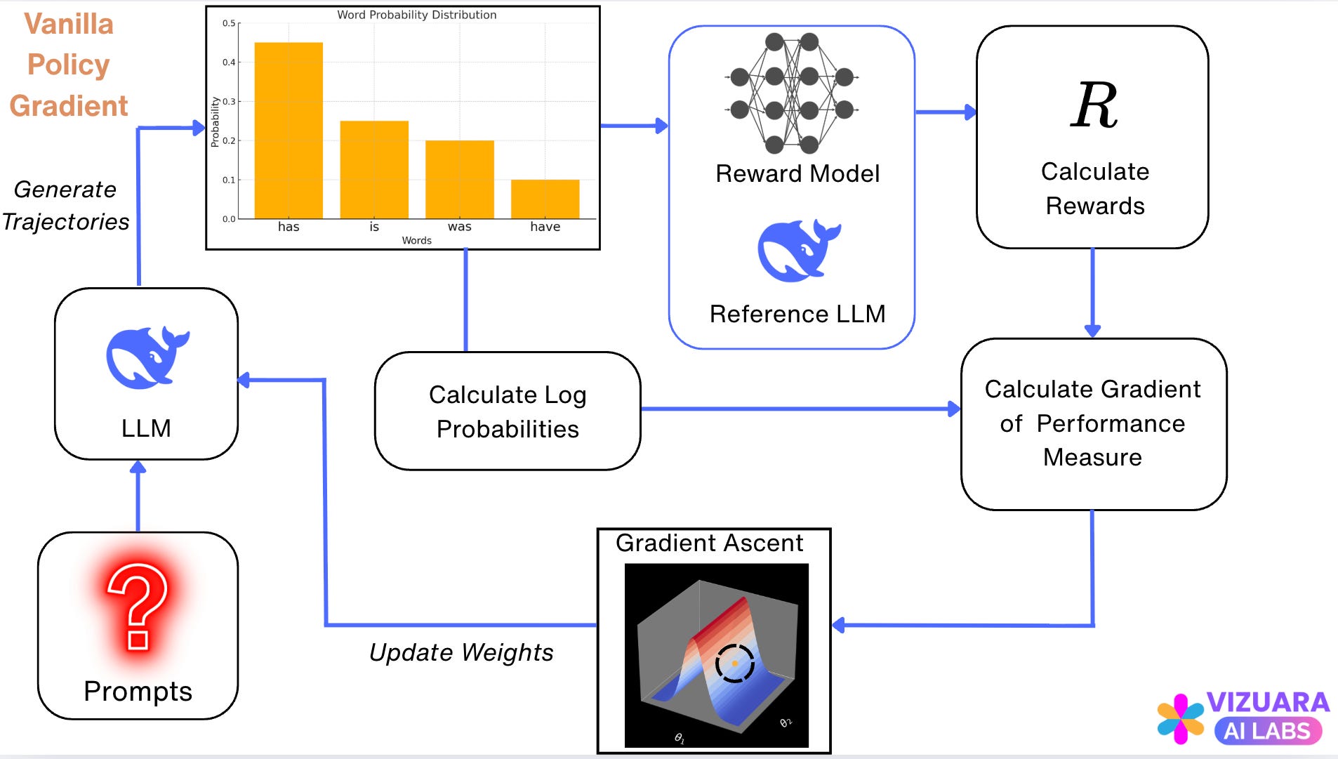
Let us go through all the steps shown in the above flowchart.
(a) Sampling trajectories
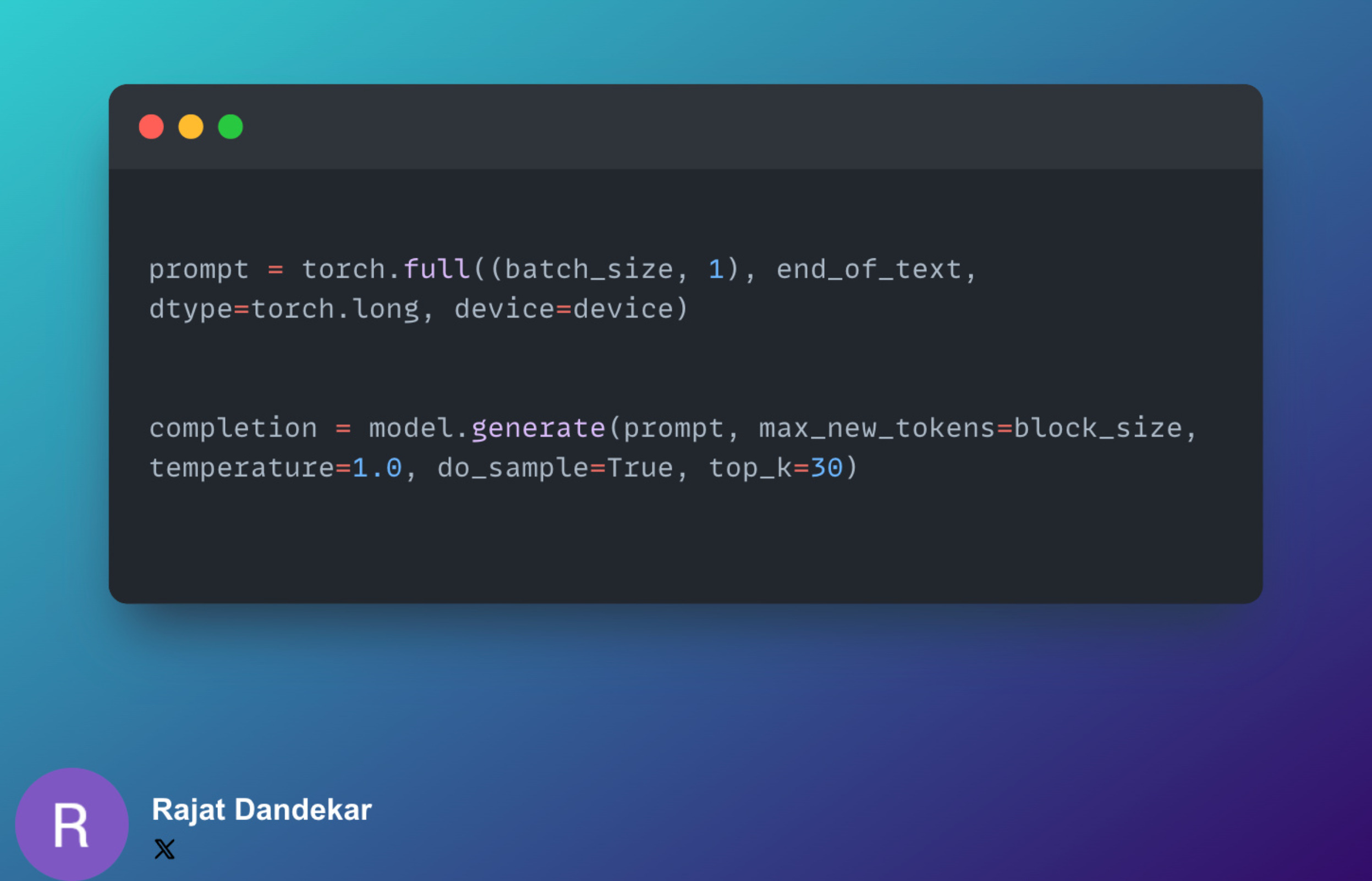
(b) Calculating the log probabilities of actions
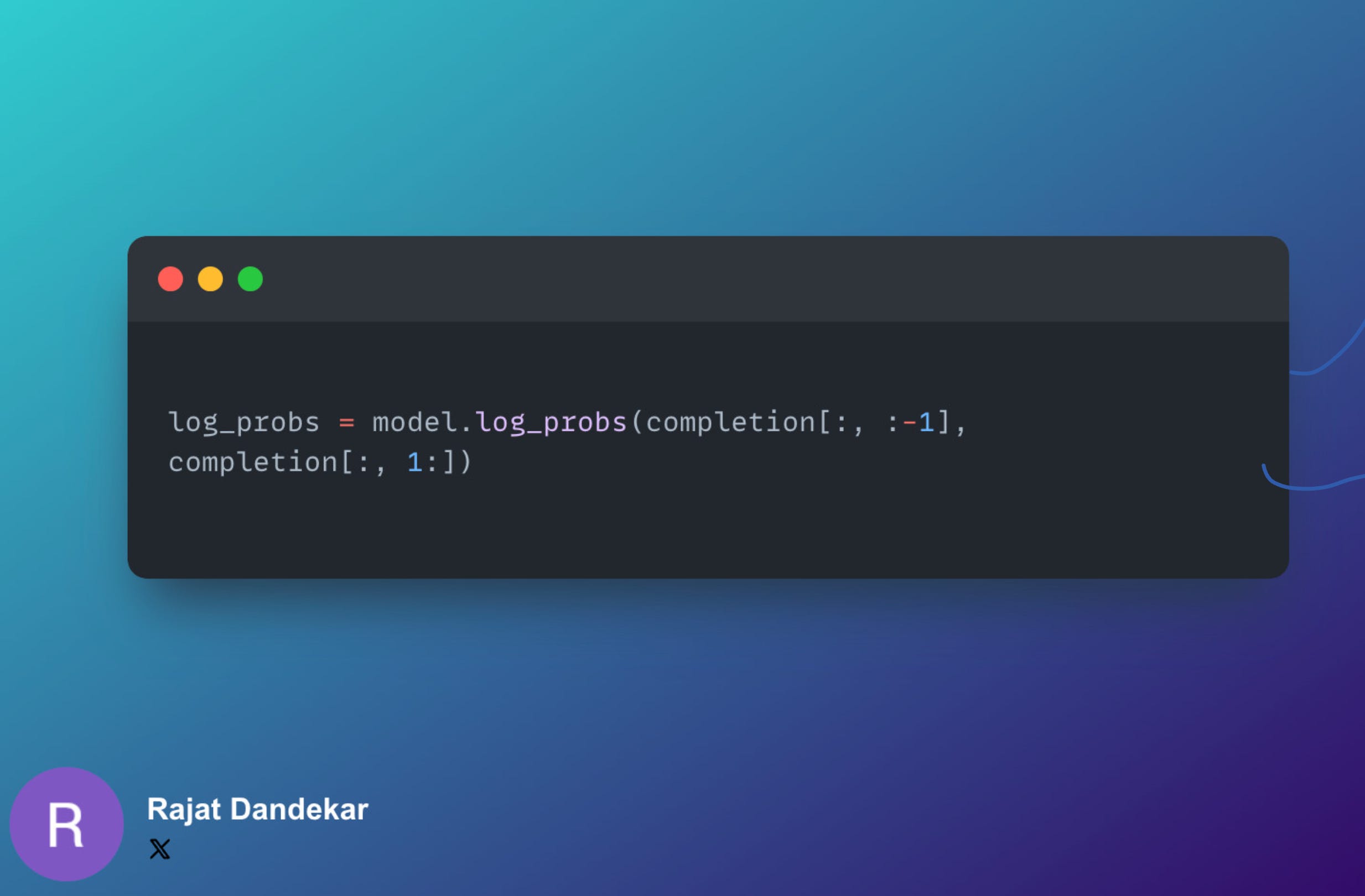
For each state, we want to find the probability of the selected action. Hence we shift the index.
Let us see why this works:
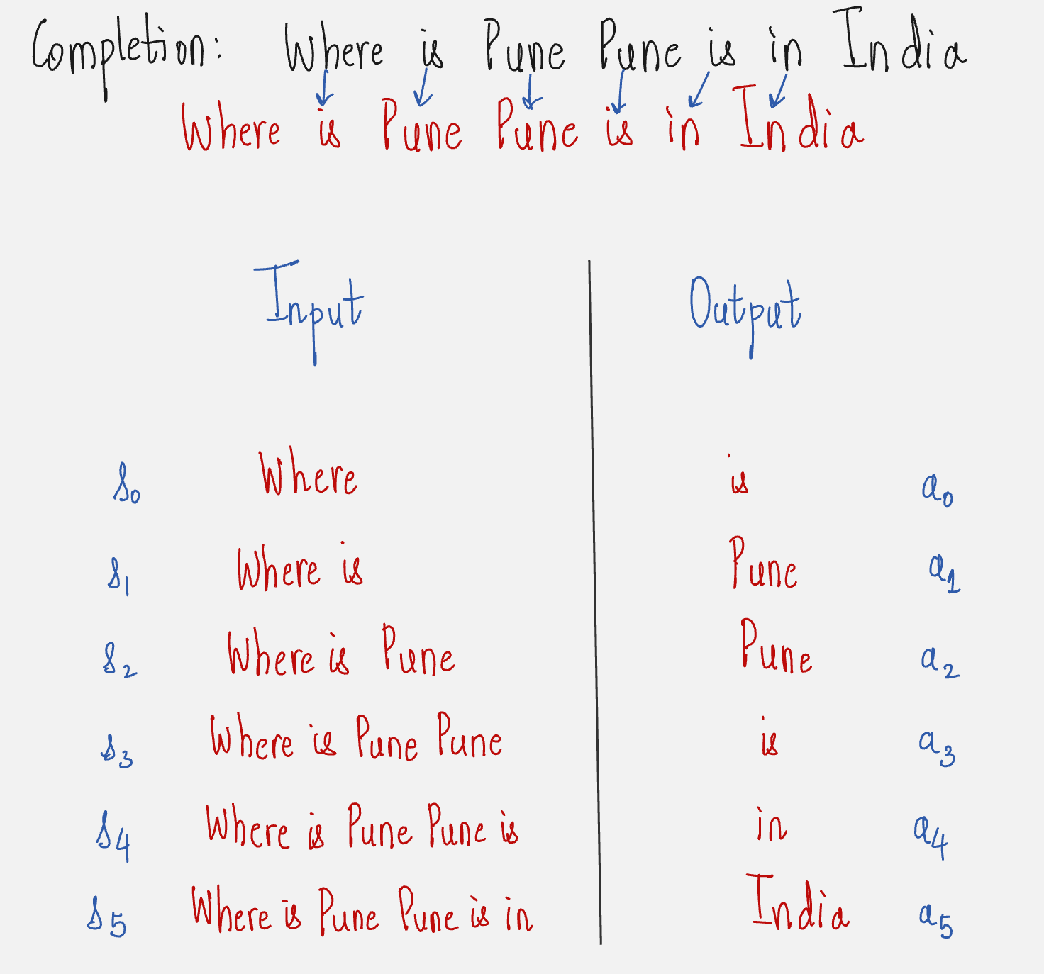
The above figure illustrates that why shifting the index works for creating input-output pairs.
(c) Calculating the rewards
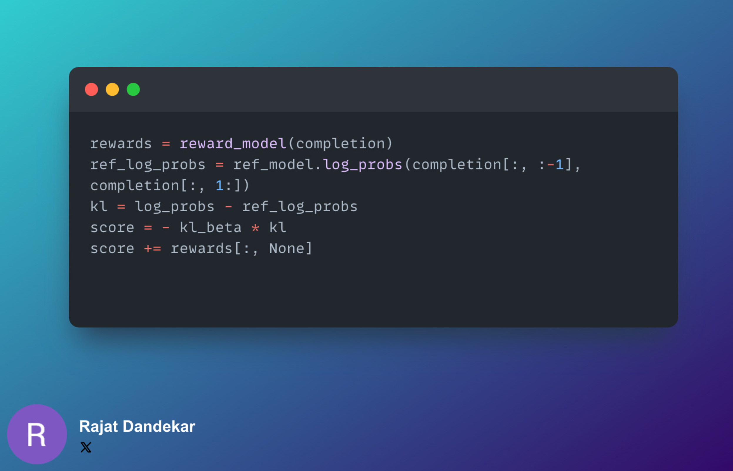
First, the reward for the entire completion is calculated. Let us call this R.
Then, the difference in the model and the frozen model's log probabilities are calculated to prevent reward hacking.
Let us see how the rewards are calculated for the example we had taken in step (b).
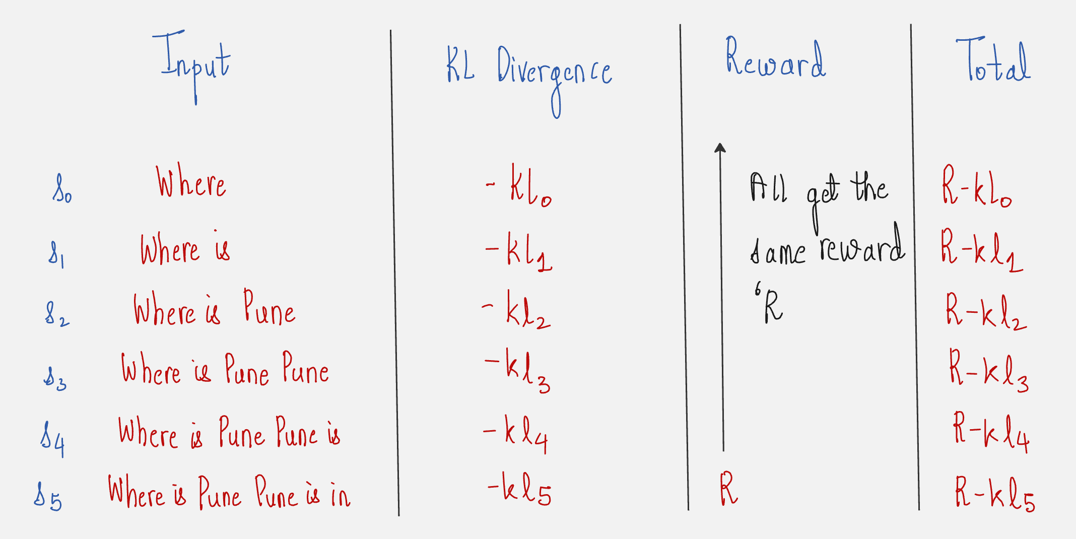
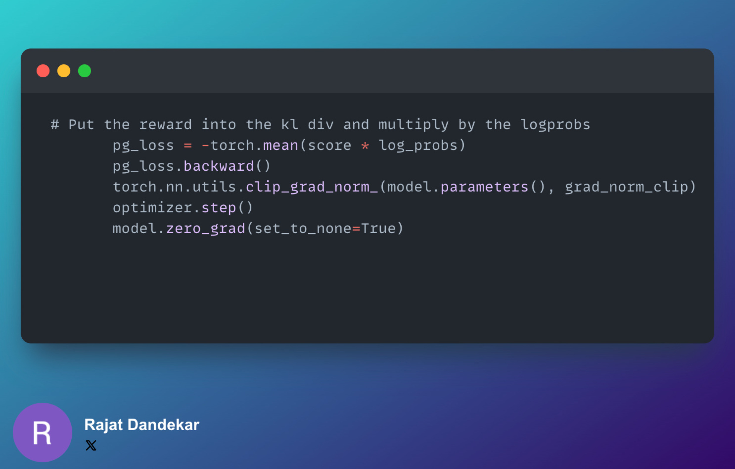
(d) Train via Vanilla Policy Gradient
(e) Results
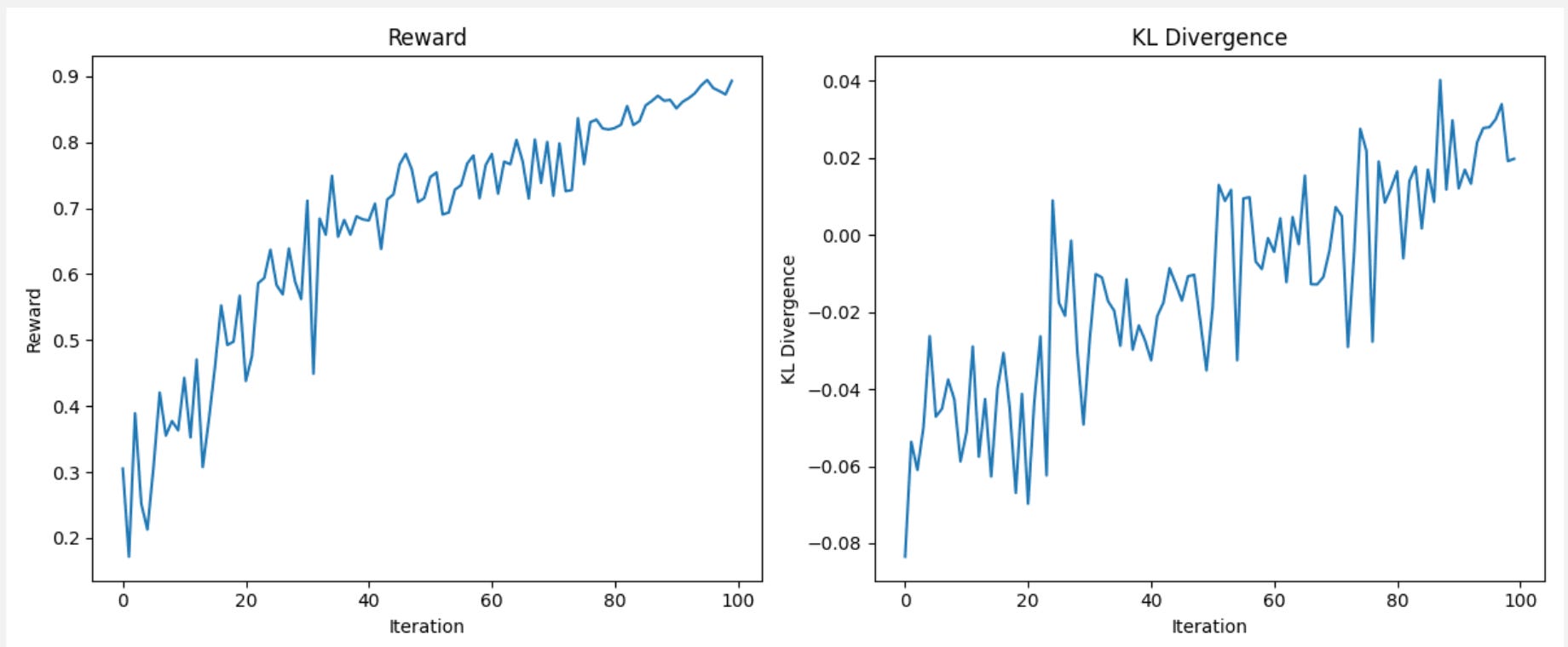
We can see that the reward is clearly rising with iterations, which means that our training is working perfectly.
We get outputs which look something like this:
Awesome!
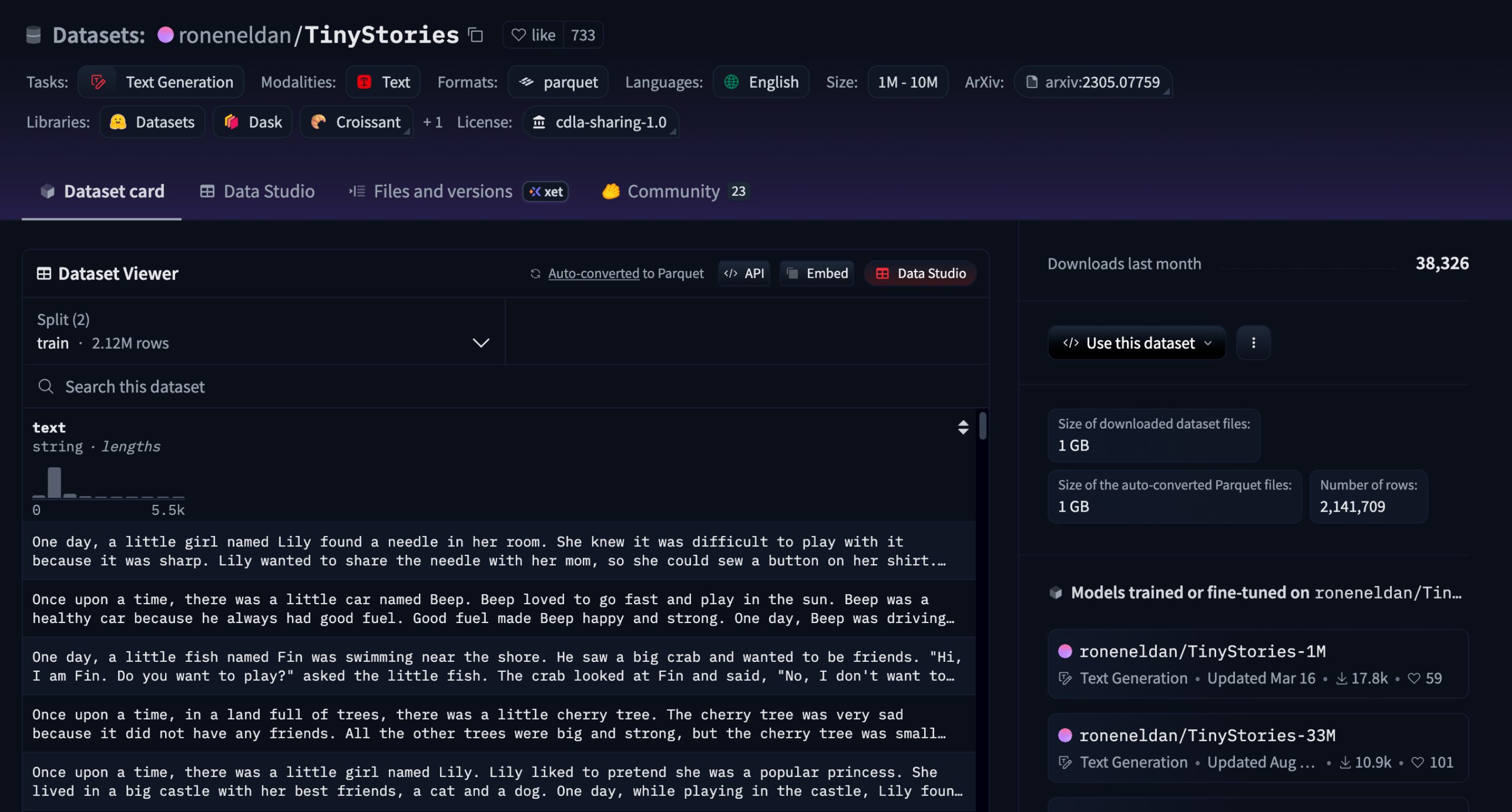
I did not stop at this. I used the same approach to train a GPT-2 model from scratch using the Tiny Stories Dataset.
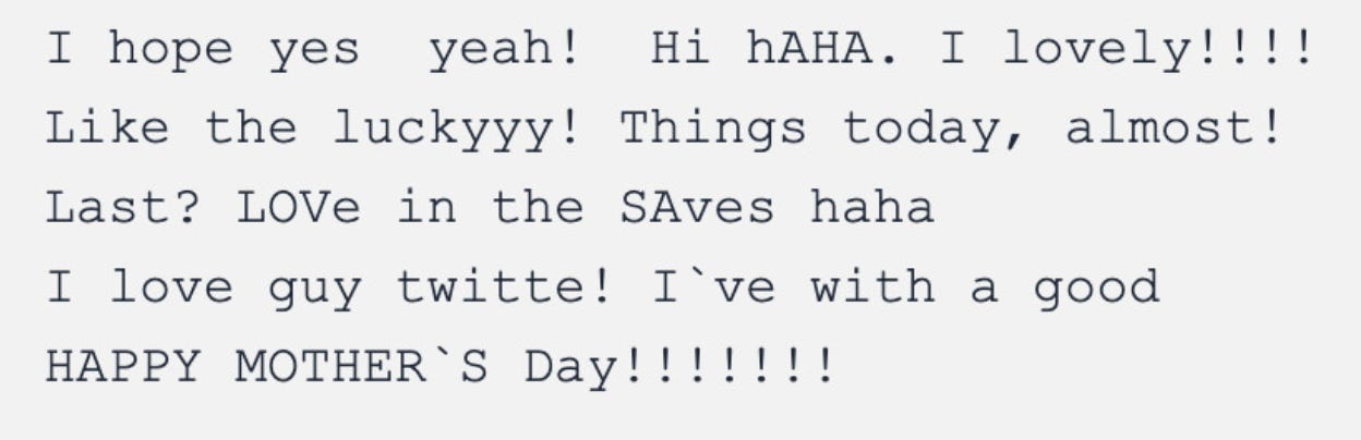
Then, I fine-tuned this model on positive stories from the dataset and used Reinforcement Learning with the Policy Gradient method to further steer the model to produce positive stories.
This result was awesome. Have a look at the positive stories that the model is able to generate (positive sentiments are highlighted in yellow):
You can use this GitHub repo for replicating this project: https://github.com/RajatDandekar/Hands-on-RL-Bootcamp-Vizuara
Navigate to the “RLHF-Part 1 Folder” and run “tinystories_pg_gpt.py” under “happy_gpt” folder.
Now let us proceed to understand another policy gradient algorithm which is common in modern RLHF implementations.
First, let us understand the concept of importance sampling.
Importance Sampling:
Notice that in the above example, while calculating the gradient of the performance measure, we have to sample a lot of trajectories.
What we are doing is optimizing our LLM and then sampling trajectories, and then again optimizing the LLM. This process continues while we train our LLM using the policy gradient method.
However, this is not a good idea because every update would require running the policy in the environment again, which is very expensive in real-world tasks. If we need thousands of updates, and each update needs new trajectories, training would take a very long time.
It would be much better if we could reuse the trajectories collected by an older policy.
This is done by a technique called as importance sampling.
Let us take a simple example to understand this.
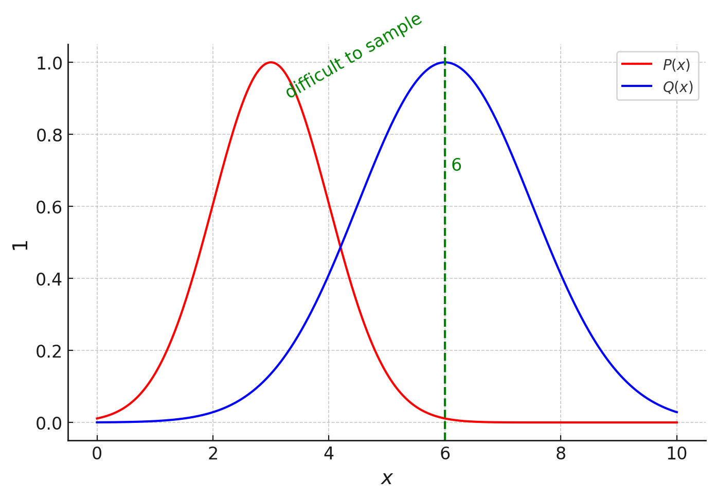
Suppose we have two distributions P and Q, and P is the distribution that we want to sample from, but it is very difficult to sample from this distribution.
We are interested in finding the expected value of x under the distribution P, which seems to be somewhere around 3.
Since it is difficult to sample from P, sample from Q instead. But the problem is that if we sample from Q, we will get the expected value of x as 6.
This is where off-policy sampling method comes in. It tells us that you can go ahead and sample from Q, but make sure to re-weight by the ratio P(x) divided by Q(x).
So if we multiply each sample from Q by the ratio P/Q, the expected value will also be multiplied by the same ratio, and so we will get the right expected value as 6*(3/6) = 3.
In summary, since it is difficult to sample from a policy which is being trained, we generate the trajectories offline and then use them for training.
To do this, we need to update the gradient of the performance measure using the importance sampling technique.
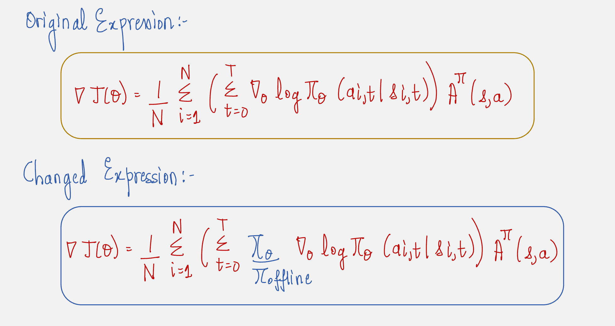
Notice how we have multiplied the original expression by the ratio of the current policy and the old policy, which is similar to P(x)/Q(x) discussed in the previous example.
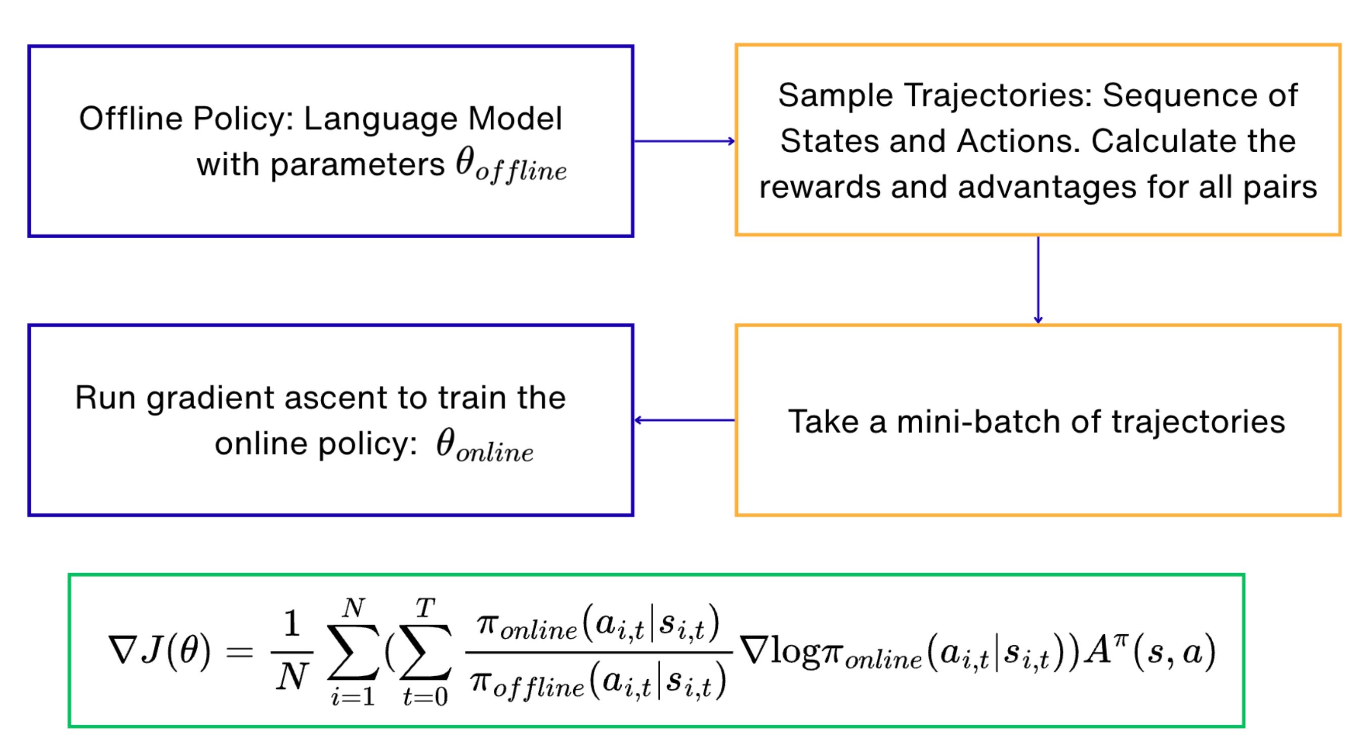
The Policy Gradient algorithm can be implemented using the following workflow:
Now let us look at Proximal Policy Optimization, which is the algorithm used in modern RLHF implementations.
Proximal Policy Optimization (PPO):
When PPO came along, we had methods which involved simple calculations, but not effective - Vanilla Policy Gradients, and methods which were effective, but involved complex calculations-TRPO.
PPO came along and said, “I will give you best of both the worlds”
Best of the first world:
PPO did not involve any constraint. The problem formulation was very similar to vanilla policy gradient methods.
Best of the second world:
PPO introduced the idea of “clipping” the policy updates, if they move beyond a specified limit.
Let us understand this with the help of an example:
Imagine that you are a runner who is trying to improve daily.

You have an “old style” of running, which is your current way of moving. You are also exploring a “new style” of running which helps you run faster. You have a coach who is giving you feedback on your performance.
This is how your learn using PPO:
Step 1: Collect Experiences (Run Daily)
You run a few laps using your current running style.
Step 2: Get Feedback from Coach (Estimate Rewards):
Your coach watches and gives feedback on how well you ran today. You compute advantage (A) which measures how better or worse is your running compared to your expected running.
Step 3: Compare New vs Old Style:
The ratio between the new style and the old style is written as:
Step 4: Did the new style actually help?
Multiply this ratio by the advantage.
Step 5: Clip Wild Changes (Coach Intervenes)
Coach says: “Don’t change too much, even if it looks better”
This avoids extreme changes in your running style.
This can be mathematically written using the clip function:
The simplicity of this algorithm proved very effective in aligning large language models to human preferences and hence it is used in modern RLHF implementations.
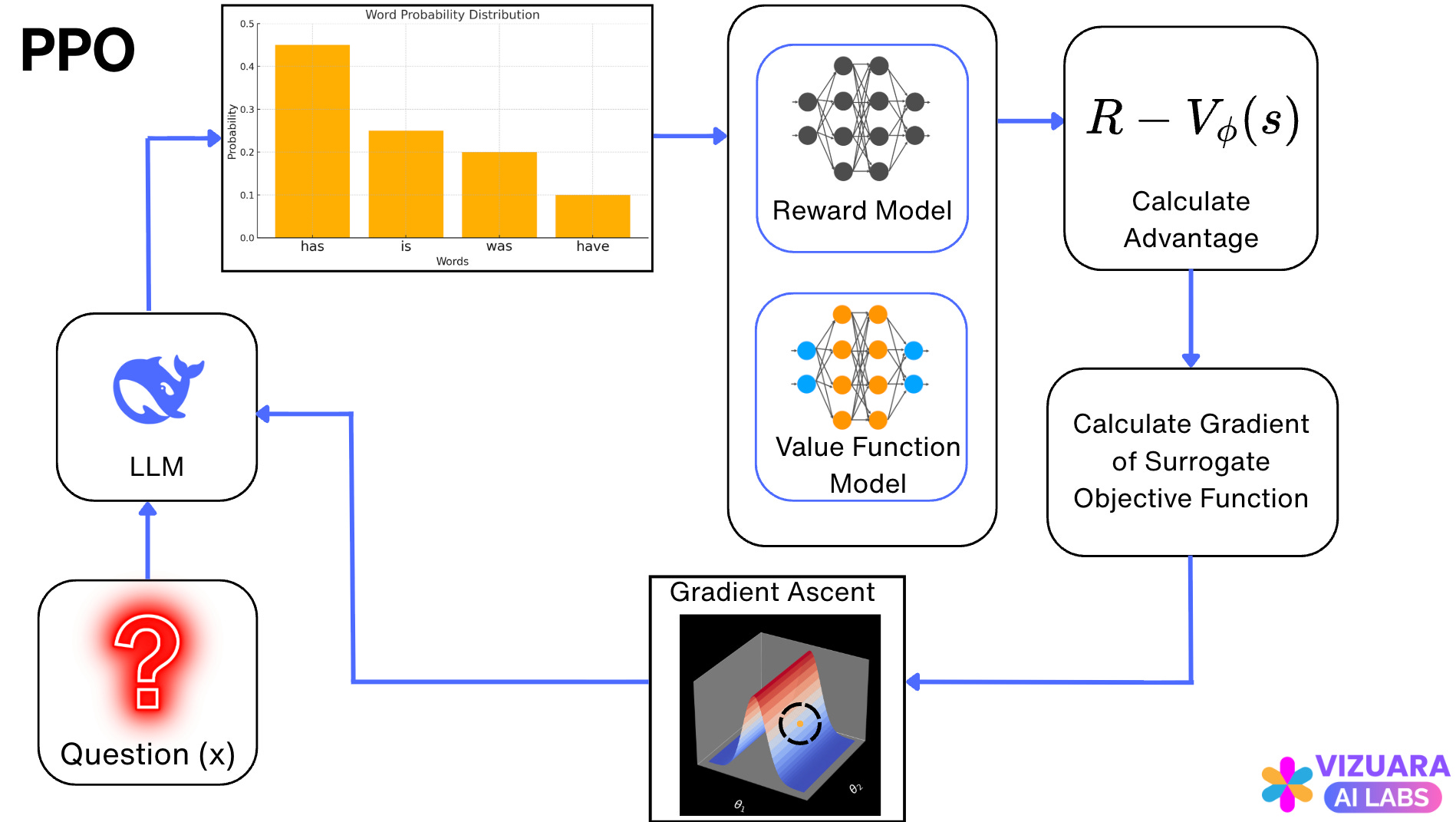
The Reinforcement Learning step using the PPO algorithm looks as follows:
Now, let us look at a practical example where PPO is used in RLHF.
Text Summarization using RLHF
We will use one of the earliest preference fine-tuning task - Reddit Post Summarization.
We will use a pretrained 124M GPT-2 model.
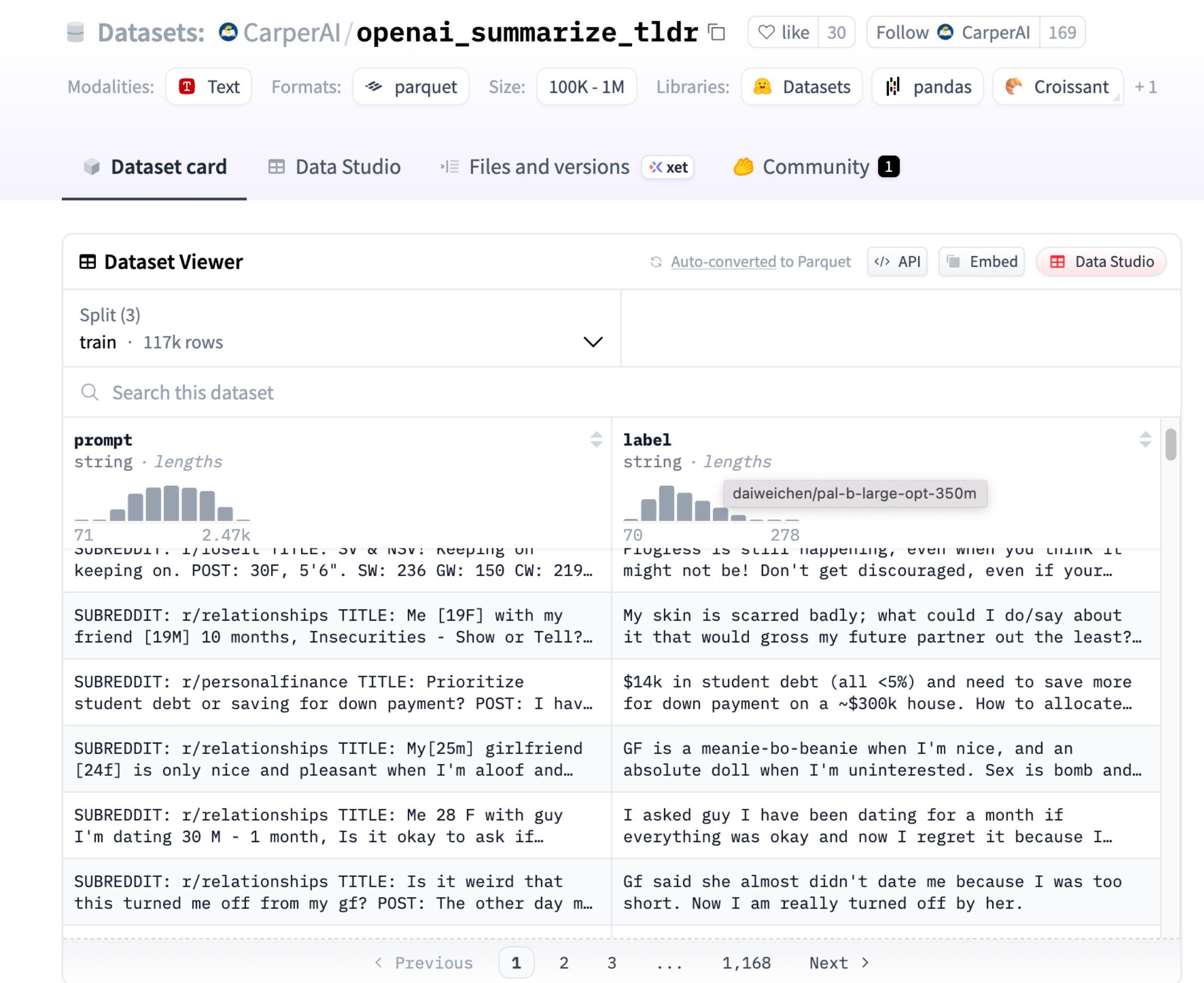
Step 1: Supervised Fine-tuning
Dataset Used:
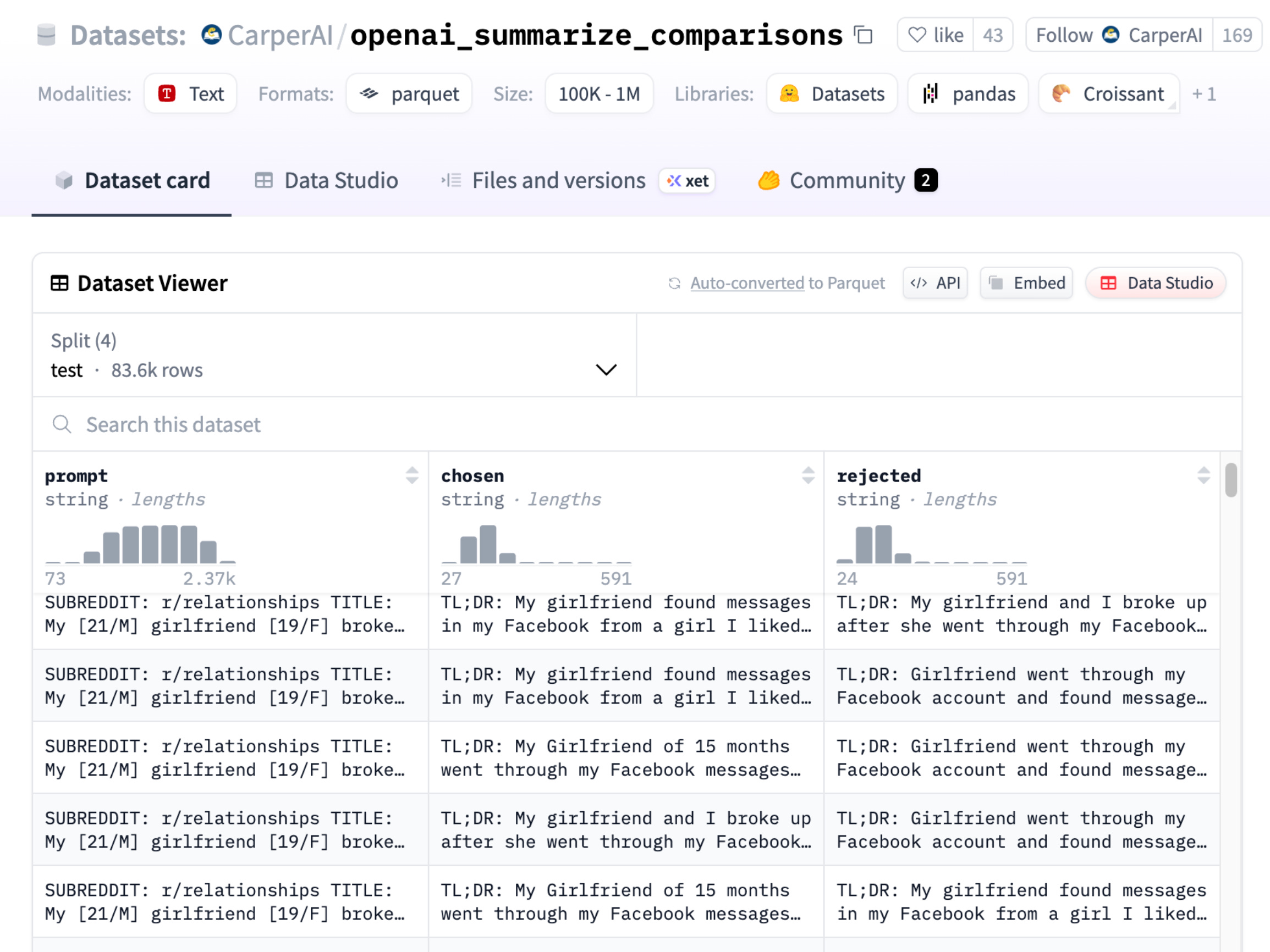
Step 2: Reward Model Training
Dataset Used:
Step 3: RL Fine-tuning using PPO
Step 4: Final Application
You can use this GitHub repo for replicating this project: https://github.com/RajatDandekar/Hands-on-RL-Bootcamp-Vizuara
Navigate to the “RLHF-Part 1 Folder” and run the 3 files for supervised fine-tuning, reward model training and PPO fine-tuning under “summarize_rlhf” folder.
Below, I am going to show an entire pipeline of how RLHF works by utilizing an interactive visualization tool that we have developed.
Regarding the topic, brilliant breakdown. Reward quantificaton feels central.