
TurboQuant: Online Vector Quantization with Near-optimal Distortion Rate
What if you can quantize your KV cache. It is the silent memory killer in long-context LLMs; TurboQuant solves it with rotation, optimal codebooks, and 1-bit residuals and proves it's near-optimal.

Table of contents
Introduction
Introduction
Every few months, the AI research world finds itself at a familiar crossroads: models are getting smarter, but the cost of running them keeps climbing. More parameters, longer contexts, heavier compute. The usual response? Throw more GPUs at it.
But there’s a quieter revolution happening in parallel, one that doesn’t ask for more resources, it asks for less. A revolution built around one deceptively simple question: how little information do we actually need to represent something meaningful?
We’ve been exploring this question together for a while now. In our 4-bit LLM training article, we started from the ground up; what is precision?, why does it matter?, what happens when you reduce mantissa bits? and how engineers handle the chaos that follows?. Then in the 1-bit LLMs article, we pushed that question to its logical extreme like what does a model look like when each weight can only say yes, no, or nothing? And how did BitNet and BitNetV2 manage to make that work without the whole thing collapsing?
Both of those articles shared a common thread: they were about quantizing the model; hence, compressing the weights, the parameters, the learned knowledge baked into the network. And they worked, remarkably well.
But here’s the thing nobody talks about enough.
Even a perfectly quantized model, running at 1-bit precision, still has to think. And thinking, in the transformer world, means attention. Attention means keys and values. And keys and values, as context grows longer, become their own memory problem; one that model quantization alone doesn’t solve.

This is where TurboQuant comes in. And it’s doing something fundamentally different from everything we’ve discussed before.
TurboQuant isn’t about compressing what the model knows. It’s about compressing what the model remembers while thinking which is the KV cache, the running ledger of keys and values that attention maintains across every token it has ever seen. As we discussed in the Kimi-Linear article, KV caching is a necessary evil. Remove it and you’re back to recomputing attention from scratch at every step, which is orders of magnitude more expensive. Keep it and it balloons with every token, eating memory that scales with context length, not model size.
So the question TurboQuant asks is sharp and specific: can we quantize the KV cache itself, not as an afterthought, but as a principled optimization problem, with theoretical guarantees about what we lose and what we keep?
The answer, as we’ll see, isn’t just yes. It’s an answer that comes with a beautiful mathematical argument for why its approach is provably better than naive quantization at the same bit budget. And to get there, it reaches into some surprisingly elegant territory that is rotation, Gaussian distributions, Johnson-Lindenstrauss projections, and a residual trick that turns the limits of quantization into an advantage.
In this article, we’ll try to build TurboQuant from scratch, the same way we’ve approached everything else here: starting with the why, building up the tools, and letting the methodology emerge naturally from the problem. By the end, the math won’t just make sense; it’ll feel inevitable. Let’s start with why quantization is such a big deal, and why the KV cache is the next frontier.
(Side note : The informtion in this article is upper bounded by a function of my knowledge/grasp on the topic, expressiveness and verboseness of my writing, the delta between my expression/writing and thought/understanding, my mood to type for hours and a writing medium that doesnt support inline latex. Hence; I would encourage you to re-visit every thing you read/learn here.)
2. A Quick Primer on Bit Representation
If you’ve read our earlier deep-dive on 4-bit LLM training, some of this will feel familiar. Think of this as a focused recap of just the pieces TurboQuant builds on; if you haven’t, this section has everything you need.
2.1 How Numbers Live Inside a Computer
Every number your model works with every weight, every activation, every key and value in the KV cache is stored as a sequence of bits. The question is: how many bits, and how are they arranged?

Floating point numbers, which are the standard currency of deep learning, are split into three parts:
Sign bit : is this number positive or negative? One bit, straightforward.
Exponent : how large or small is the number, in terms of powers of 2? This controls the range of values you can represent.
Mantissa : the fractional precision, the fine-grained detail within that range.
A helpful way to think about this: imagine you’re describing a location on a number line. The exponent tells you which neighbourhood you’re in; it places you coarsely on the line, somewhere between 0.001 and 0.01, or between 10 and 100. The mantissa then tells you exactly where inside that neighbourhood you are. More mantissa bits = more precise location within the neighbourhood. Fewer mantissa bits = you can only point to a rough spot, not an exact address.
This maps directly onto something we use every day. In scientific notation, the number π ≈ 3.14159265358979323846... is written as 3.14159265358979323846…. × 10⁰.

The part before the decimal that is the 3; is the coarse location. The part to the right of the decimal .14159265358979323846... is the mantissa. It’s the fractional residue that carries the fine-grained information.
In coordinate geometry, if you think of a number line as an x-axis, the exponent places you at a position along that axis (the abscissa the horizontal distance from the origin), while the mantissa is like the sub-division of that position, the fractional part that sits within the unit interval at that location. Two completely different ideas, but they illuminate the same underlying structure: coarse placement first, fine detail second.

FP32 gives you 23 mantissa bits and 8 exponent bits. BF16 trades mantissa precision for speed; it keeps the same 8 exponent bits (so the range stays large) but cuts the mantissa down to 7 bits. INT4 goes further still, with essentially no mantissa at all just 4 bits of integer range.
2.2 Why Reducing Mantissa Shrinks the Model but Costs You Information
Here is the core tension that every quantization paper is wrestling with.
Fewer bits = less memory. A weight stored in FP32 takes 32 bits. The same weight in INT4 takes 4 bits is an 8× reduction. At the scale of billions of parameters, this is the difference between a model that fits on one GPU and one that requires eight. So the pressure to reduce bits is real and enormous.
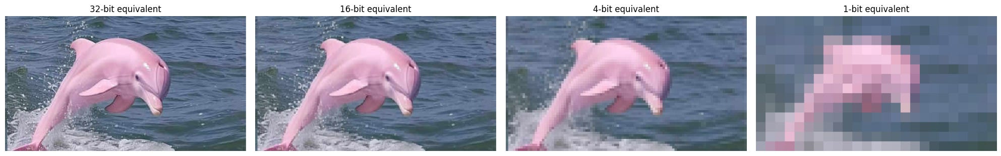
But every bit you remove from the mantissa is a resolution you’re giving up permanently. Values that were once distinct; say 0.7312 and 0.7318; now round to the same bucket. The model can no longer tell them apart. And unlike lossy image compression where you might not notice a blurry background, in a neural network these small distinctions compound. A gradient that was 0.003 might round to zero. A key vector that was subtly different from its neighbour might become identical. Multiplied across billions of parameters and thousands of forward passes, these small rounding errors accumulate into meaningful drift.
This is not just a storage problem. It’s an information geometry problem. When you quantize, you are partitioning a continuous space into a finite number of buckets, and everything that falls into the same bucket becomes indistinguishable. The fewer the bits, the larger the buckets, the coarser the partition, and the more information irreversibly collapses.
The mantissa is precisely where this collapse happens. The exponent controls which part of the number line you’re on, as soon as you reduce it; you lose range (which is not desirable). But reduce the mantissa, and you lose resolution within each range; which is painful but more tolerable, because in large distributed systems, each individual weight doesn’t need to be infinitely precise. The collective effect of many imprecise weights can still approximate a good function, especially when the weights are spread across many dimensions.
This is the bet that quantization makes. And up to 4-bit, as we saw in earlier articles, it’s a bet that largely pays off for model weights.
The KV cache, however, is a different story and that’s exactly what makes TurboQuant’s approach necessary. We’ll get to that shortly.
3. Quantization on KV Cache
Before we get into what TurboQuant does, we need to deeply understand the problem it’s solving. This section is about building that conviction; why the KV cache specifically?, why quantizing it is different from quantizing weights, and why it’s become the next big thing.
3.1 Two Places You Can Quantize an LLM
When we talk about making LLMs more efficient through quantization, there are really only two places to intervene: the weight space and the token space.
Weight space is what we’ve been discussing in our earlier articles. The model’s learned parameters are composed of the billions of floating point numbers baked in during training which are then compressed to lower precision. This is a one-time cost. You quantize the weights once, and you carry that compressed model everywhere (Techniques like BitNet, QLoRA, GPTQ have been covered here).
Token space is different. This is the space of activations; the intermediate computations the model performs as it processes each new token at inference time. These aren’t fixed like weights as they’re generated fresh for every new input, and they grow with every token the model sees. This is where the KV cache lives.
Now, the research community has done an admirable job on weight space quantization. We have robust methods, strong theoretical understanding, and production-grade implementations that let us run models at 4-bit or even 1-bit with surprisingly little quality loss. That problem, while not fully solved, is reasonably well understood. Token space quantization and specifically KV cache quantization is where the real uncharted territory begins and the reason it matters is scale.
3.2 Why the KV Cache Gets So Large
Let’s make this concrete. Every transformer layer maintains a cache of keys and values for every token it has processed. This is the mechanism that lets the model attend to past context without recomputing it from scratch. As we discussed in the Kimi-Linear article, this is not optional it’s the thing that makes autoregressive generation tractable at all. But the cost is memory, and that grows without bound.
For a model with L layers, H attention heads, head dimension d, and a context of n tokens, the KV cache size is:
The factor of 2 is for keys and values separately. Everything else is fixed by architecture; except n (context length), which grows with every token generated. At 128k context, a single LLaMA-70B layer’s KV cache can rival the size of the model weights themselves. Across all layers, it easily exceeds them.
This means two things. First, the KV cache is often the dominant memory cost at inference, not the model weights. Second, unlike weights which you compress once offline, the KV cache must be compressed online, token by token, at inference speed. That constraint fundamentally changes what methods are viable.

3.3 KV Caching Is a Necessary Evil
Here is a thought experiment worth sitting with. What happens if you simply don’t cache the KV pairs?
Every time the model generates a new token, it would need to recompute the full attention over all previous tokens from scratch. The keys and values for every past token would need to be recomputed by re-running them through the model. For a context of n tokens, this means O(n) full forward passes just to generate one new token. The compute cost becomes quadratic O(N^2) in context length; this is exactly the problem the KV cache was invented to solve/avoid.
So removing the cache entirely is not a real option. It would push the cost back into weight-space compute, multiplied by sequence length, and that product grows catastrophically. The KV cache is the mechanism by which we offload that quadratic cost into linear memory. It is, in the truest sense, trading memory for compute. A necessary evil.
Which means the question isn’t whether to have a KV cache. It’s how to make the one we have as small as possible, without losing what attention actually needs from it.
3.4 Why This Problem Is Different from Weight Quantization
You might reasonably ask: if we can quantize model weights to 4-bit with good results, why not just do the same thing to KV cache entries?
The answer is that KV cache vectors and model weights have very different statistical properties, and quantization methods that work well for one tend to work poorly for the other.
Model weights, after training, settle into distributions that are relatively well-behaved roughly Gaussian, with moderate outliers that can be managed. They’re also static. You can study their distribution offline, design a codebook around it, and apply it once.
KV cache vectors are dynamic. They’re produced by the model as it processes each new token, and their distribution shifts with every input. A key vector generated while processing a legal document looks nothing like one generated mid-conversation. Outliers appear unpredictably, distributions are non-uniform across dimensions, and the whole thing changes at inference time when you have no opportunity for offline calibration.
This is precisely why naive quantization of the KV cache like applying INT4 or INT8 as you would to weights; leads to noticeable quality degradation. The buckets you designed for one distribution are wrong for another. Information collapses in the exact dimensions where attention needs it most.
TurboQuant’s central insight is that this isn’t a quantization problem to be patched; it’s an optimization problem to be solved properly. And solving it properly requires a completely different framework, one that doesn’t assume anything about the shape of the input distribution, but instead transforms the data into a shape where quantization can be applied optimally. That framework is what we build next.
4. Quantization as a Constrained Optimization Problem
This is where TurboQuant stops being just another compression trick and starts being something more interesting. We’re going to reformulate the entire quantization problem from scratch; not as an engineering patch, but as a mathematical optimization with a well-defined objective. Once you see it this way, everything that follows in the methodology feels inevitable.
4.1 Finding the Right Transformation
Let’s start with the most general possible framing. Lets say you have a matrix A, which is a block of key vectors from your KV cache, stored in full precision. You want to find a compressed version B, stored in far fewer bits, such that the information loss is minimized. Formally, you’re looking for a transformation G such that:
and the difference between A and G(A) is as small as possible in some meaningful sense.
But what does “meaningful sense” actually mean here? This is the question most quantization papers gloss over, and it’s where TurboQuant takes a sharp turn. The naive answer is mean squared error.
Simple, differentiable, easy to optimize. But MSE treats all errors as equally bad, regardless of direction. A large error in a dimension that attention never looks at costs the same as a tiny error in a dimension that attention relies on completely. That’s clearly wrong.
The right objective, once you think about it is this: preserving verboseness/variance, while minimising bits required to represent the information; which is basically our well-known cross entopy. This is a rate-distortion problem. Minimize distortion (error in attention scores; represented by a inner-product) subject to a bit-rate constraint (how many bits you’re allowed to use).
Formally, if q is a query vector and k is a key vector, what you care about preserving is:
where k_hat is the quantized version of k. Every design choice in TurboQuant flows from this single objective. Found this intuitive? No? Don’t worry, this will be discussed in-depth in upcoming sections.
4.2 Bits as Dimensions of Information
Here’s a reframing that makes the optimization problem much cleaner to think about. Each bit you allocate is an additional dimension of information. A 1-bit representation can distinguish two states. A 2-bit representation can distinguish four. An N-bit representation carves your space into 2^N distinct buckets.
Now think about what this means geometrically. Your key vector k∈R^d lives in a d-dimensional space. Quantization is the act of partitioning that space into 2^N regions and assigning every vector in the same region the same code. The quality of your quantization depends entirely on how well those regions align with where your data actually lives.
This is where the connection to principal components becomes natural. If your data has high variance along certain directions and near-zero variance along others; which is almost always true for real activation vectors, then the optimal partition should allocate (in ideal case) more resolution to the high-variance directions and less to the low-variance ones. The directions of maximum variance are exactly the eigenvectors of the covariance matrix. Each principal component is, in a very real sense, the most informative dimension to allocate a bit to.
So the optimization problem becomes: find the transformation G that, before quantization, rotates your data so that the bits you have are spent on the dimensions that carry the most information. Not uniformly. Not blindly. But Adaptively, according to where the variance is maximum. This is the core of TurboQuant, and everything else is working out the details of how to do this efficiently.
4.3 The Problem with Fixed Codebooks
Most existing quantization methods like INT4, BF16, NF4 which work with a fixed/static codebook. A codebook is just a lookup table (that contains our range) and our G function maps our domain/input to this range. Algorithmically; it is a pre-defined set of 2^N values that every quantized number must be mapped to. You find the nearest codebook entry to your input, store its index, and call it done. In practical cases, these could should be thought of as eigen matrix (where codebook vectors are principle components); but due to unavailability of known domain of input, we can’t do that.

The problem is that these codebooks make an assumption about the shape of your data. INT4 assumes uniform spacing across a fixed range. NF4, as we discussed in the QLoRA context, assumes a normal distribution. These assumptions are baked in at design time, before anyone has seen your specific data.

For model weights, this is acceptable. Weights are roughly Gaussian after training, and you can verify this offline. But for KV cache vectors, as we established in the previous section, the distribution is dynamic, non-uniform, and shifts with every input. Any static codebook will be wrong for at least some inputs and wrong in exactly the dimensions attention cares most about.
There’s a deeper issue too; in high-dimensional spaces, data rarely distributes uniformly across all dimensions. It clusters along a few principal directions a low-dimensional manifold embedded in a high-dimensional space. When you apply a uniform codebook to such data, you’re spreading your resolution budget evenly across all dimensions, most of which contain almost no information. The result is that the dimensions that actually matter; i.e. the principal directions get the same resolution as the noise dimensions (that’s a terrible allocation).
What you really want is a codebook that adapts to the data’s geometry; something that concentrates resolution where variance is high and vice versa. The way to achieve that (as we’ll see in the methodology), is to first transform the data into a space where the distribution is approximately uniform and known, apply the optimal codebook for that known distribution, and then handle whatever the transformation couldn’t capture with a second, complementary step.
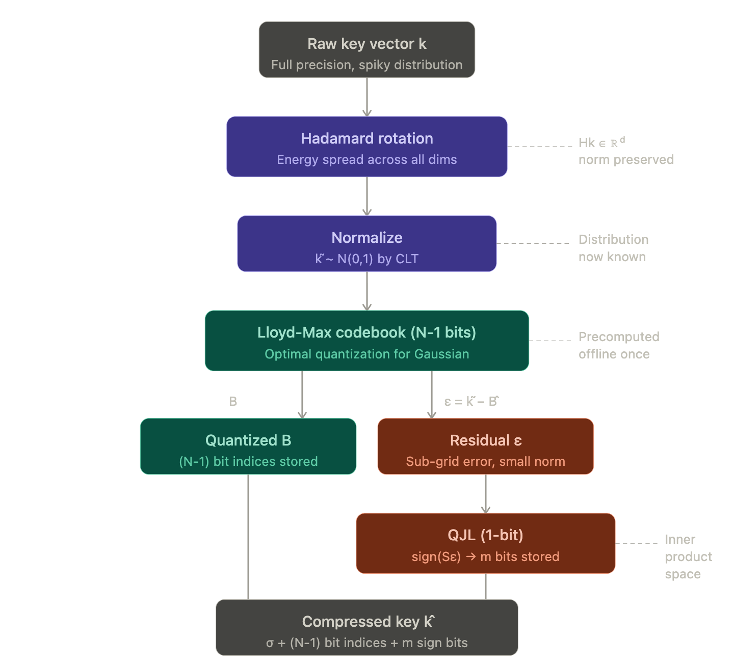
That two-step structure : transform then quantize (which is where the vector is; handled through MSE based TurboQuant) + handle the residual (which direction the vector points; handled through inner-product based TurboQuant) separately is the architecture of TurboQuant’s solution. We’ll build it piece by piece in the next section.
5. Methodology
This is where everything we’ve built so far the optimization framing, the codebook problem, the geometry of high-dimensional data; all comes together into an actual algorithm. We’ll take it in two parts. First, how TurboQuant transforms the problem into one it can solve optimally. Then, how it handles what’s left over (residual) through QJL .
5.1 Solving the Unknown Distribution Problem (MSE persepective)
Recall where we ended up in Section 4. The fundamental difficulty with quantizing KV cache vectors is that their distribution is unknown, non-uniform, and shifts with every input. Any fixed codebook will be misaligned with the data’s actual geometry, wasting resolution on low-variance dimensions and starving the dimensions that attention actually depends on.
TurboQuant’s answer to this is elegant: don’t try to design a codebook for an unknown distribution. Instead, transform the data into a known distribution, and design the optimal codebook for that. The target distribution is Gaussian. Here’s why that choice is not arbitrary.
5.1.1 The Residual Decomposition
Lets start with the fundamental decomposition that frames the entire methodology:
where A is your original full-precision key vector, B is the quantized approximation, and ε is the residual; the information that quantization failed to capture. The task is to minimize ε, and TurboQuant attacks this in two complementary stages that together give you N bits of total representation.
The transformation G handles the first stage:
G transforms A into a known distribution B which is easier to quantize and work with. The only condition is that G must be bijective/invertible; because if it isn’t, you’ve already destroyed information before quantization even begins. The next question is what G should do to make the quantization of B as lossless as possible.
5.1.2 Getting into a Known Space via Rotation
The first thing G does is apply a rotation to the input vector. Why rotation specifically? Because rotation has a property that no other transformation shares for this purpose: it is norm-preserving. For any orthogonal matrix R:
The total energy of the vector; i.e. the sum of squared values across all dimensions; is unchanged. What rotation does is redistribute that energy. A vector that had most of its energy concentrated in 2 of 8 dimensions, after a well-chosen rotation, can have its energy spread more evenly across all 8.
This redistribution matters enormously for quantization. Remember, a fixed codebook allocates equal resolution to every dimension. If your data is spiky then high variance in a few dimensions, near-zero in the rest; then equal resolution allocation is a terrible fit. Most of your bits are spent describing near-zero dimensions, and the high-variance dimensions get the same coarse treatment as everything else. After rotation, the energy is spread; each dimension now carries a more comparable amount of information, and equal resolution allocation starts to make sense. By rotating we are not corrupting the vector; because during inference when we apply the same randomized rotation matrix for decoding / reverse the rotation; then we get the original vector back (almost).
Why does rotation specifically give a Gaussian distribution? This is where the Central Limit Theorem earns its place. The Hadamard rotation matrix which is the specific rotation TurboQuant uses has a beautiful structure: each output dimension is a sum of all input dimensions, weighted by ±1/d. Concretely, for a d-dimensional input vector k:
Each rotated dimension is a sum of many terms. By the Central Limit Theorem, the sum of many independent (or weakly dependent) random variables converges to a Gaussian distribution, regardless of the original distribution of the individual terms. So even if the raw KV cache vector had a spiky, non-uniform, pathological distribution, after Hadamard rotation its dimensions are approximately N(0,σ^2).
Hence, the domain is now known which is a normal distribution; and a known domain means you can precompute the optimal codebook offline.
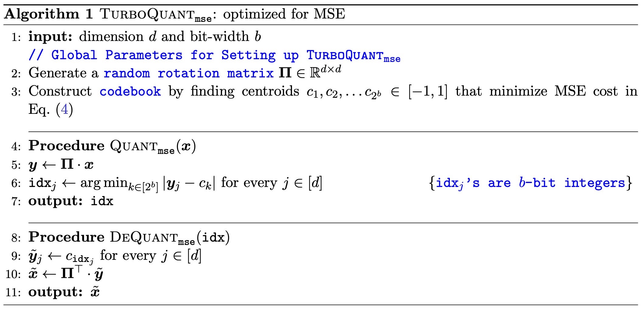
5.1.3 Precomputing the Optimal Codebook via Lloyd-Max
Once you know your data is approximately Gaussian, the codebook design problem has a clean, classical solution: the Lloyd-Max algorithm.
Lloyd-Max finds the MSE-optimal quantization thresholds and reconstruction levels for any known distribution. For a Gaussian, these are fixed constants as they depend only on the number of bits N and the variance σ^2, both of which you can estimate or normalize for. Concretely, for an N-bit codebook, Lloyd-Max gives you 2^N thresholds {t1,t2,…,t2N−1} and 2^N reconstruction levels {r1,r2,…,r2N} such that the expected squared error is minimized over the Gaussian distribution.
The key point is that these thresholds are precomputed once and reused for every vector. You do the offline work once, and at inference time, quantization is just a lookup; find which threshold bin the rotated value falls into and store the bin index. This is both theoretically optimal for the Gaussian distribution and practically fast.
The MSE perspective (Lloyd-Max + rotation) here is solving the storage problem. Given a vector, how do you represent it in fewer bits such that the reconstructed vector is as close as possible to the original in Euclidean distance? This is a Cartesian problem as it lives in the coordinate space of the vector itself. The rotation + Gaussian + Lloyd-Max pipeline is the optimal solution to this specific problem. It minimizes ||k−k^||2
This solves the transformation G for the main body of the information. But G optimizes MSE in a fixed known space, and MSE in Cartesian coordinates is not the same as preserving inner products. There will be a residual ε which are small, but non-zero and that represents the gap between what the codebook can express and the true vector. And as we’re about to see, the way TurboQuant handles that residual is where things get genuinely interesting.
5.1.4 Example
Let’s make this concrete with a worked example. Real KV cache head dimensions are typically 64, 96, or 128. We’ll use d=8 to keep the arithmetic readable while preserving the qualitative behavior of the high-dimensional case.
Take a raw key vector in full precision:
Notice the structure: most energy is in dimensions 1, 4, and 6, with near-zero values everywhere else. This is typical of real attention key vectors, as they have sparse energy, not uniformly distributed.
Step 1 — Hadamard Rotation
Apply the normalized 8×8 Hadamard matrix H. Each output dimension becomes a ±1/sqrt(8) weighted sum of all inputs. The result, approximately:
The energy that was concentrated in three dimensions is now spread across all eight. The values are roughly comparable in magnitude as no single dimension dominates. The distribution of these values across many such vectors would be approximately N(0,σ2) by CLT.
Step 2 — Normalize to N(0,1)
Estimate σ from the rotated vector (or from a running estimate across recent vectors). Divide through:
Now each component is approximately standard normal.
Step 3 — Apply Lloyd-Max 3-bit Codebook
For a standard Gaussian, the 3-bit Lloyd-Max thresholds are approximately:
with 8 reconstruction levels at the conditional means between each pair of thresholds. Mapping each component of k^ to its nearest reconstruction level:
storing 3 bits × 8 dimensions = 24 bits, plus a scalar σ in 16-bit = 40 bits total for the main quantization.
Residual:
Small; but not zero. This residual contains the fine-grained directional information that the codebook’s fixed grid couldn’t capture. And this is exactly what Section 5.2 will handle, using QJL to compress it into a single additional bit per projected dimension, in a way that is provably better than simply allocating those bits to the main quantization instead.
5.2 Handling the Residual with QJL (inner-product perspective)
We have the main quantization done. The rotation spreads the energy, the Lloyd-Max codebook captures most of it optimally, and what remains is a small residual vector ε. The question now is: what do you do with it? And why is the answer compressing it with a completely different kind of tool is provably better than just throwing more codebook bits at the original problem?
5.2.1 Why the Codebook Alone Isn’t Enough
Let’s think carefully about what ε is.
After the Lloyd-Max quantization, ε is the vector of errors the difference between the true normalized key vector and the nearest codebook reconstruction. Geometrically, ε lives in the gaps between codebook grid lines. It’s the sub-grid residue that the quantizer couldn’t represent because the grid isn’t fine enough.
The obvious response is: just add more bits. Go from 3-bit to 4-bit quantization. The grid becomes finer, the gaps shrink, and ε gets smaller.
This is correct, but it’s not the whole story. And here’s the subtle point TurboQuant makes: adding another codebook bit reduces ε in the MSE sense, but MSE is not what attention cares about. Attention cares about inner products; specifically, whether M and N are close enough; These are related but not identical objectives.
More concretely: the residual ε after (N−1)-bit quantization has a specific geometric structure. It lives in directions that the codebook, by construction, cannot represent the sub-cell directions, orthogonal in some sense to the quantization grid. Adding a N-th bit to the codebook refines the grid, but the refinement happens in the same Cartesian geometry as the original quantization. The directions the codebook couldn’t represent at N−1 bits are still the directions it struggles with at N bits; they’re just slightly smaller.
QJL operates in an entirely different geometric space; which is the inner product space and that orthogonality of approaches is precisely what makes the combination powerful.
5.2.2 Johnson-Lindenstrauss: The Theory Behind the Projection
Before getting into the sign quantization step, it’s worth understanding what the Johnson-Lindenstrauss (JL) lemma actually guarantees, because TurboQuant’s theoretical claims rest on it directly.
The JL lemma states: for any set of vectors in Rd, there exists a random projection matrix S∈R of (m×d) dimensions with m≪d, such that for any two vectors u,v:
with high probability, where each entry of S is drawn i.i.d. from N(0,1/m).
In plain language: a random projection preserves inner products in expectation, up to a bounded error that shrinks as m grows. The projection is lower-dimensional; you go from d dimensions to m dimensions; but the geometric relationships between vectors in inner-product space are approximately maintained (the things that are close remain relatively close after the transformation; remeber UMAP, TSNE?)

This is the key property TurboQuant needs. Because attention scores are inner products between queries and keys, and JL projections preserve inner products, you can work in the projected space and still recover approximate attention scores. The randomness of S provides the guarantee; not any specific structure, just the statistical property of Gaussian random matrices.
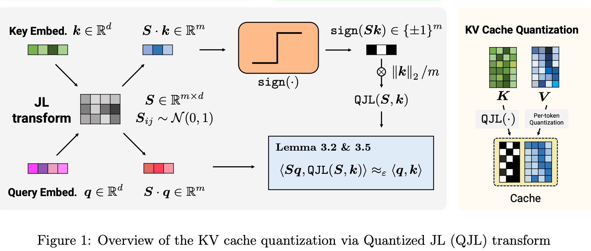
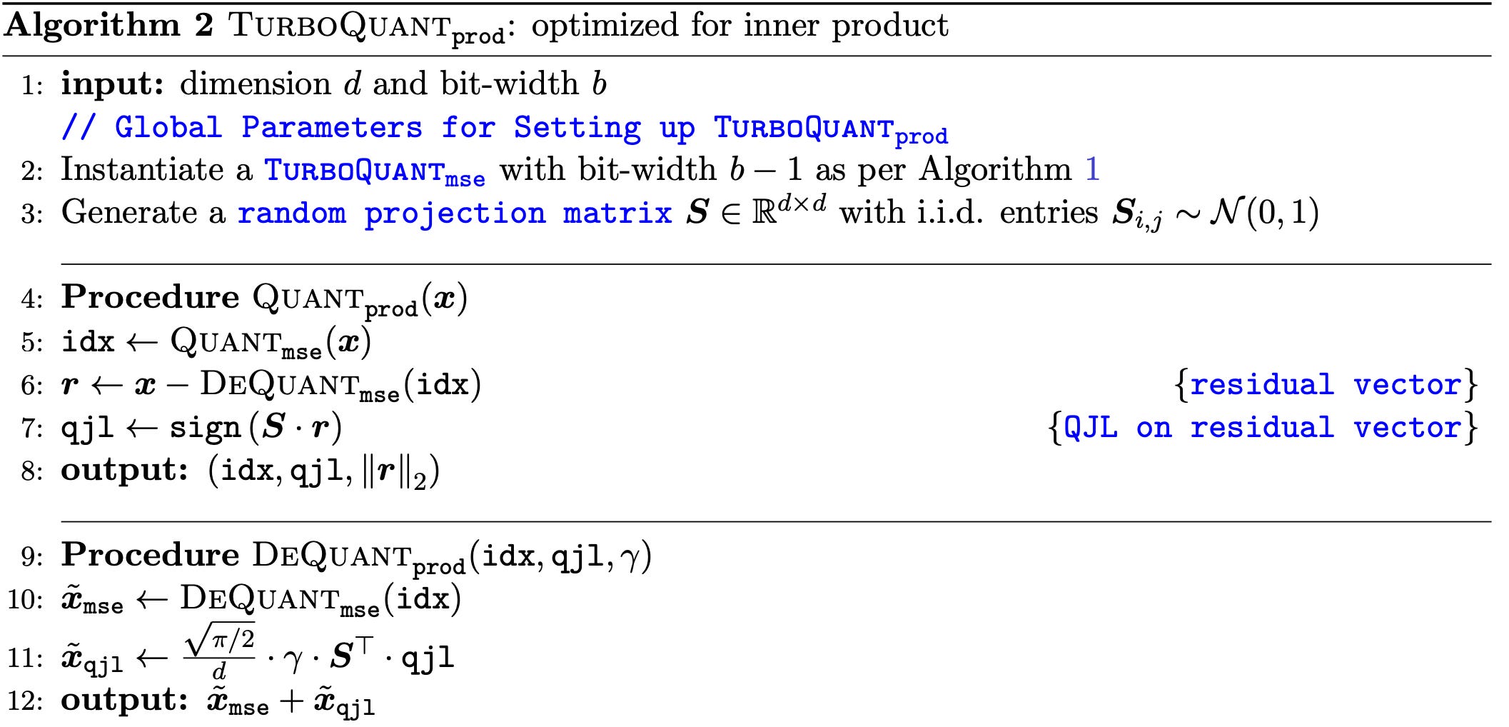
5.2.3 QJL: Random Projection Meets 1-Bit Quantization
QJL combines the JL projection with the most aggressive quantization possible: storing only the sign of each projected dimension. The procedure is straightforward. Given the residual vector ε∈Rd:
Step 1 — Project:
where S∈Rm×d is a random Gaussian matrix, fixed at initialization and shared across all tokens. This is a one-time cost.
Step 2 — Quantize to 1 bit:
Store only the sign of each projected dimension; this results in m bits total. That’s it. The entire residual is compressed to m bits, regardless of the original dimension d.
Why Does Sign Quantization Still Preserve Useful Information?
Think about this as a search problem. Imagine a large grid of people standing in a field. You’re trying to locate where a specific person is standing, but you can’t look directly. Instead, you can ask other people in the field a single binary question: did you find them on your left or your right?
One person’s answer is almost useless. They might be standing at an awkward angle where even two people far apart look like they’re on the same side. But ask enough people, each standing at a different random position in the field, and something remarkable happens; the pattern of left/right answers starts to triangulate the target’s location. More people answer the same way → the target is nearby. Answers are evenly split → the target is far, or in the opposite direction entirely. This process helps in reconstructing the entire manifold/matrix/nodes from relations/edges.

This is exactly what sign quantization does to vectors. Your high-dimensional vector space is the field. Every possible key vector is a person standing somewhere in it. Each random projection vector si is someone you're asking and their specific position gives them a unique perspective on the space, determining what they consider "left" versus "right." The sign bit is their answer. And Hamming agreement the fraction of people who give the same answer about two different targets tells you how close together those targets are standing.
Lets looking it from a more geometrical viewpoint;
Imagine two vectors in 2D; an arrow pointing mostly right, and another pointing mostly right-and-slightly-up. They’re similar. The angle between them is small.
Now imagine a random line through the origin. When you project both vectors onto this line, you get a number which is positive if the vector points “with” the line, negative if it points “against” it. The question is: do both vectors land on the same side?
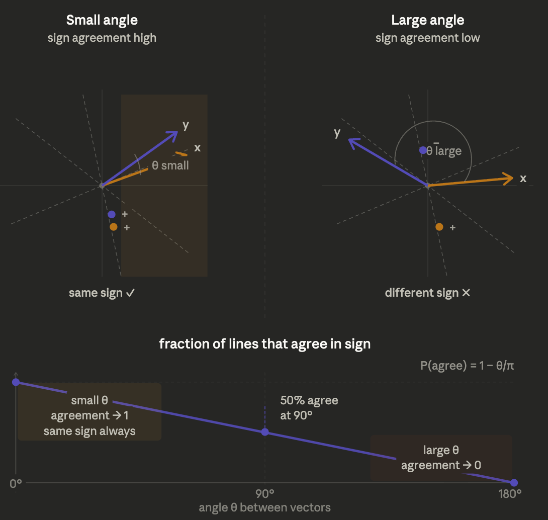
If the angle between the two vectors is small then they’re nearly parallel which means almost any random line will put them on the same side. They’ll both be positive, or both be negative. Sign agreement is high.
If the angle is large then they point in opposite directions which means many random lines will separate them. One lands positive, one lands negative. Sign agreement is low.
If they’re exactly perpendicular (90° apart) then exactly half the random lines will agree, half will disagree.
This is the key insight: the fraction of random lines on which two vectors agree in sign is a smooth, monotonic function of the angle between them. More similar vectors → more sign agreement. More different vectors → less sign agreement.
Why This Recovers the Inner Product
The inner product q⊤k can be decomposed as:
Three things: the magnitude of q, the magnitude of k, and the angle between them.
QJL’s sign bits directly encode cosθ whic is the angular part. Here’s how:
You draw m random Gaussian vectors s1,s2,…,sm
For each one, you record whether si⊤q and si⊤k have the same sign
The fraction of agreements across all mm m vectors estimates 1−θ/π, which is a direct function of cosθ
So from the sign bits alone, you can recover the angle. And if you also store ||K|| separately (which TurboQuant does, via the scale factor σ), you have everything you need to reconstruct q⊤k.
Simple Example
Say q=[1,0] and k=[0.9,0.1] almost the same direction, small angle between them.
Draw a random vector s=[0.6,0.8]
s⊤q=0.6 → positive
s⊤k=0.54+0.08=0.62 → positive
Same sign. ✓
Draw another: s=[−0.3,0.95]
s⊤q=−0.3 → negative
s⊤k=−0.27+0.095=−0.17 = −0.175 → negative
Same sign. ✓
Now try q=[1,0] and k=[−0.9,0.1] nearly opposite directions, large angle.
Draw s=[0.6,0.8]
s⊤q=0.6 → positive
s⊤k=−0.54+0.08=−0.46 → negative
Different sign. ✗
If you repeat this many times, the fraction of agreements directly tells you how similar the two vectors are directionally. Formally, for any two vectors x and y, the probability that a random Gaussian vector s gives them the same sign is:
where θxy is the angle between them. Small angle → high agreement. Large angle → low agreement. Exactly what the field analogy predicts.
as we saw above, the inner product q⊤k decomposes into three things:
The magnitudes ||q|| and ||k|| are stored separately as scalar scale factors. The sign bits recover cosθ which is the angular part through Hamming agreement. Put them together and you have the full inner product, reconstructed entirely from binary observations.
The part that feels almost too good to be true is that you never measure distance directly. You never store magnitudes of individual projections. You throw away everything except the sign (the most aggressive compression imaginable) and yet the geometry survives, statistically, across enough random perspectives. This is why QJL error scales as 1/sqrt{m}: each additional question is an independent measurement from a new angle, and independent measurements average out their individual errors progressively.
This also explains why spending your last bit on QJL beats spending it on a finer codebook grid. Adding a codebook bit makes your existing map slightly more detailed in one region; but it refines the same Cartesian geometry the previous bits already worked in. Asking a new random person is an entirely new perspective from an independent angle reduces uncertainty everywhere simultaneously, including directions your codebook had never covered at all.
Concretely, at inference time, to estimate the attention score q⊤k using the QJL-compressed residual:
The Hamming agreement between sign vectors is a simple bitwise operation (XOR) gives an unbiased estimator of the inner product. This is extremely cheap to compute at inference time, which matters enormously for a KV cache operation that runs on every single generated token.
5.2.4 Why (N−1)-bit + 1-bit QJL Beats N-bit
This is the result that elevates TurboQuant from a clever engineering trick to something with genuine theoretical teeth. Let’s build the argument carefully.
Pure MSE quantization at N bits:
For a Gaussian source with variance σ^2, the distortion of the optimal N-bit quantizer scales as:
The improvement from (N−1) bits to N bits is:
So adding the N-th bit to the codebook reduces distortion by a factor of 3/4 of the previous level’s distortion. This is what you get from spending that extra bit on the main quantization.
QJL on the residual at 1 bit:
The QJL estimator’s error for inner product estimation is:
where m is the number of random projections (= number of sign bits stored). Crucially, this error is geometrically independent of the MSE codebook error. Here’s why: the codebook error lives in the sub-cell directions of the quantization grid(the Cartesian gaps the grid couldn’t resolve). The QJL error lives in the angular estimation error of random hyperplane projections which is a completely different geometric object. The two errors don’t share subspace.
This independence is the key. When you add a N-th codebook bit, you’re reducing error in the same space that the first N−1 bits already worked in the Cartesian MSE space. The marginal gain shrinks because you’re refining a grid that already captured most of the structure.
When you instead add QJL on the residual, you’re reducing error in a new space; whic is the inner product space where the codebook had zero coverage. The marginal gain is much larger because you’re covering territory that was previously completely unaddressed.
More formally, the combined distortion of (N−1)-bit codebook plus 1-bit QJL on the residual satisfies:
and because these errors are in orthogonal subspaces relative to the attention objective, they don’t compound. Whereas pure N-bit quantization gives:
for the inner product preservation objective, whenever mm m is chosen appropriately relative to d. The theorem in the paper makes this precise with explicit constants, but the intuition is clean: spending your last bit on a completely different geometric tool covers more ground than spending it on refining the same tool you already have.
The inner product block (QJL) is solving the inference problem. Given a compressed key, how do you estimate q⊤k accurately at query time? This is not a Cartesian problem as it's an angular problem. It doesn't care how close k^ is to k in Euclidean distance. It cares whether the angle between q-k is preserved and reproducable.
5.2.5 Example
Returning to our key vector from Section 5.1.4. After 3-bit Lloyd-Max quantization, we had:
Step 1 : Sample random projection matrix
Draw S∈R(6×8 matrix), each entry is sampled from ∼N(0,1/6). Fixed at initialization, reused for every key vector. A representative S:
Step 2 : Project the residual
Step 3 : Take the sign
Stored as 6 bits: 101010.
Final storage summary:
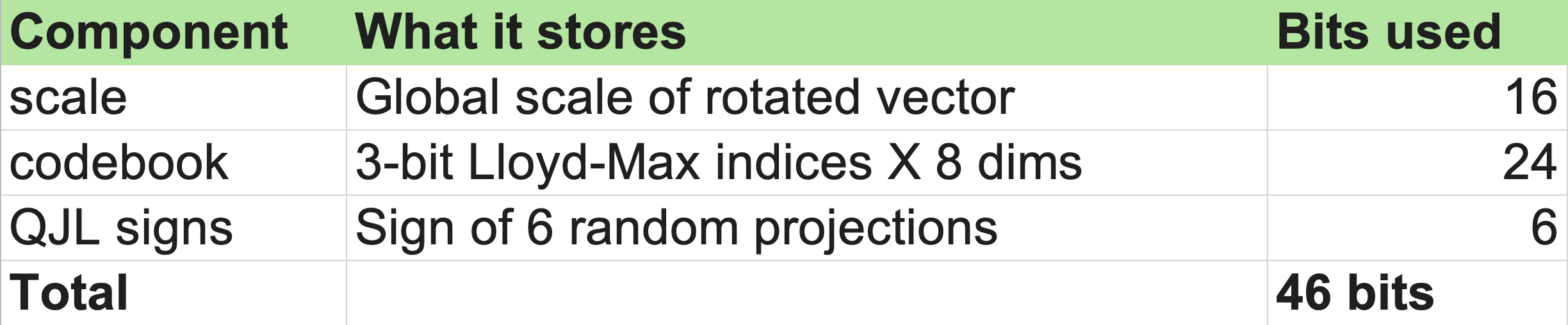
Compare to full FP32 storage: 8×32=256. That’s a 5.6× compression on this toy example. At real head dimension d=128, the compression ratio grows substantially ; the codebook scales linearly with d, but the QJL sign budget m can be held fixed or grown much more slowly, since inner product estimation error scales as 1/sqrt{m} regardless of d.
At inference, to estimate the attention score between a query q and this compressed key:
Reconstruct the main term: dequantize k^ using the codebook and scale by σ.
Estimate the residual contribution: compute sign(Sq) and take Hamming agreement with stored ε^.
Combine:
\(q^\top k \approx q^\top(\sigma \hat{k}) + \frac{\pi}{2}\|\varepsilon\| \cdot \text{HammingAgreement}(\text{sign}(Sq),\ \hat{\varepsilon})\)
Both operations are fast: the codebook lookup is a table read, and the Hamming agreement is a bitwise XOR followed by a popcount; a single CPU/GPU instruction.
6. Results & Outcomes
6.1 Theoretical Bounds Hold in Practice
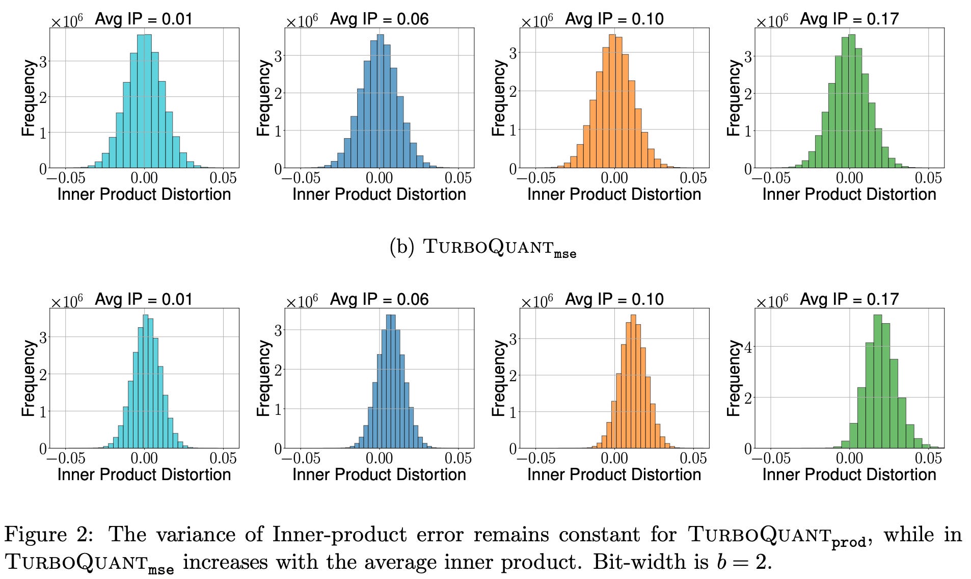
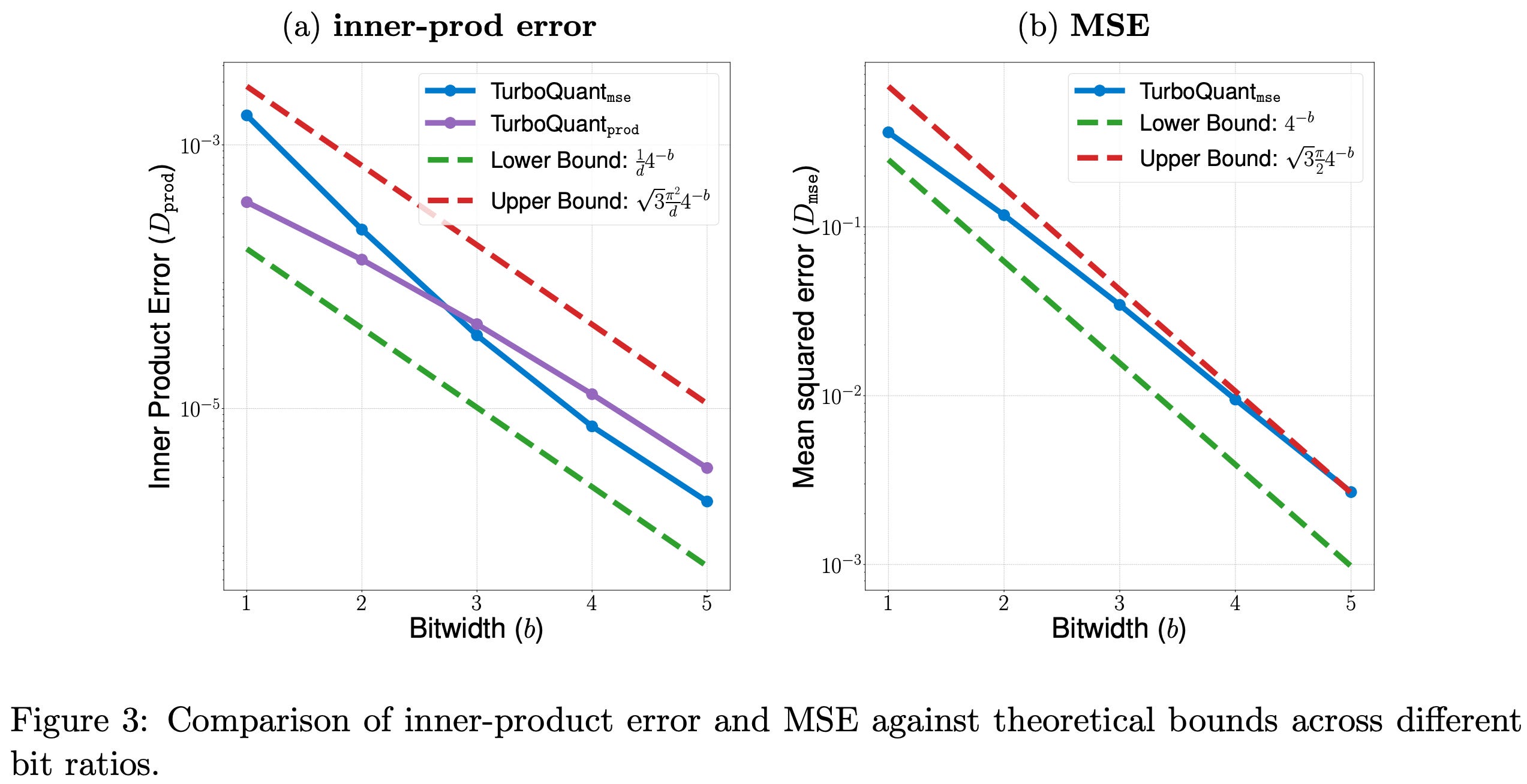
The first thing the authors validate is whether TurboQuant’s distortion actually matches what the theory predicts. Using 100,000 vectors from the DBpedia dataset encoded into 1536-dimensional OpenAI embeddings, they measure inner product error and MSE across bit-widths 1 through 5.
The results confirm two things cleanly. First, TurboQuantprod_{inner_prod} remains unbiased for inner product estimation across all bit-widths as its error distribution is centered at zero regardless of how high or low the average inner product is. TurboQuantmse_{mse}, by contrast, introduces a bias that grows with the average inner product value and only diminishes at higher bit-widths. Second, the observed distortions track tightly with the theoretical upper and lower bounds derived in the paper; the gap between TurboQuant and the information-theoretic optimum is consistently within the predicted factor of sqrt(3π/2)≈2.7.
This is important because most quantization papers validate empirically without connecting results back to theory. TurboQuant earns both.
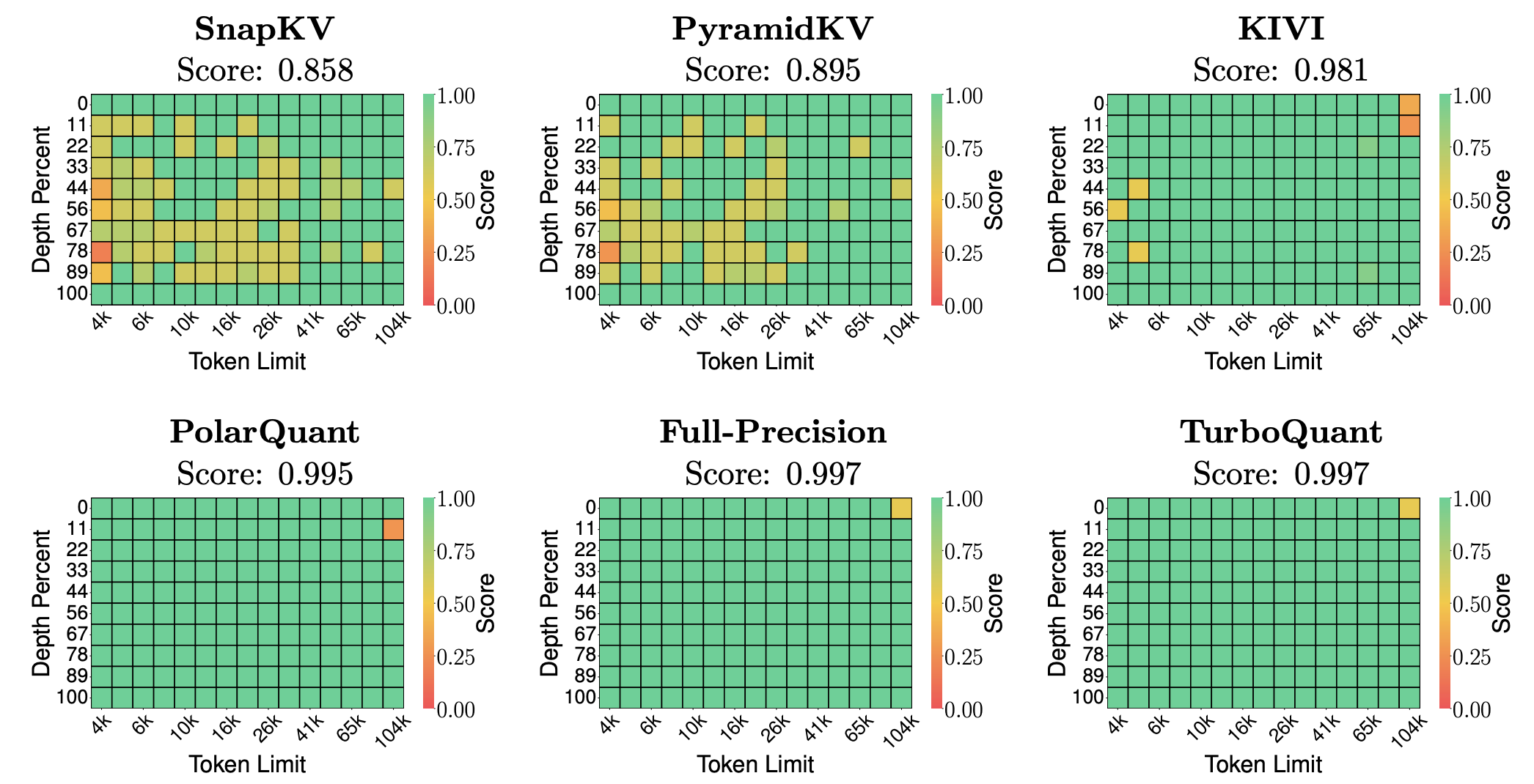
6.2 Needle-in-a-Haystack: Perfect Recall at 4× Compression
On the Needle-in-a-Haystack benchmark; where Llama-3.1-8B-Instruct must retrieve a specific hidden sentence from contexts ranging from 4k to 104k tokens; TurboQuant achieves a recall score of 0.997, identical to the full-precision uncompressed baseline, while using only 25% of the full KV cache.
For reference, the competing methods at the same compression ratio score:
This means methods without formal theoretical guarantees like SnapKV, PyramidKV; degrade noticeably as context grows. KIVI holds up reasonably but still falls short. TurboQuant matches full precision exactly, which is the result the theoretical guarantees predict: unbiased inner product estimation means retrieval tasks, which depend entirely on which key vector is most similar to the query, should be unaffected by compression.
6.3 Compression Ratios: How Much Memory Does It Actually Save?
At real KV cache head dimensions typically d=64 to d=128; the compression story is compelling.
Full precision FP16 storage for a single key vector of dimension d=128 costs 128×16=2048 bits. TurboQuant’s representation breaks down as:
Scale factor σ: 16 bits (one FP16 scalar)
Lloyd-Max indices: (N−1) bits × d dimensions
QJL signs: m bits, where mm m is chosen independently of d
At N=4 (3-bit codebook + 1-bit QJL) and m=64 random projections:
That’s a 4.4× compression over FP16, or equivalently, roughly 4-bit effective precision; matching INT4 quantization in storage cost, but with the theoretical inner product preservation guarantees that raw INT4 cannot provide.
At m=32 projections, you get:
And importantly, m can be tuned independently of d. For very long contexts where memory is the primary bottleneck, you reduce m. For tasks where attention precision is critical, you increase it, this flexibility doesn’t exist in fixed-codebook methods where every bit is committed to the same geometric space.
At the system level, a 4.4× reduction in KV cache size translates directly into one of three benefits, depending on what you optimize for: you can serve the same context length on a GPU with 4.4× less memory, or serve 4.4× longer contexts on the same hardware, or fit 4.4× more concurrent users in the same memory budget. In production serving, where KV cache is typically the binding memory constraint at long contexts, any of these is significant.
6.4 Comparison Against Baselines
On LongBench-E; which covers single and multi-document QA, summarization, few-shot learning, synthetic tasks, and code completion, TurboQuant is evaluated at two effective bit-widths: 2.5 and 3.5 bits. These non-integer values come from treating outlier channels separately, applying higher precision to the 32 most active channels and lower precision to the remaining 96.
Against naive INT4: At the same 4-bit budget, TurboQuant preserves inner products more accurately because the rotation step ensures the distribution is Gaussian before quantization, rather than applying a fixed grid to an arbitrary distribution. On tasks with long contexts and distributional shift between training and inference; exactly the cases where KV cache quantization matters most; there these gaps widens.
Against KIVI: KIVI applies group quantization with per-channel scaling, which partially addresses the non-uniform distribution problem. TurboQuant’s rotation approach is more principled; it provably Gaussianizes the distribution rather than approximately normalizing it and the addition of QJL for the residual gives it a second degree of freedom that KIVI doesn’t have.
Against KVQuant: KVQuant uses learned codebooks calibrated on representative data. This works well in-distribution but requires calibration data and can degrade on inputs that differ from the calibration set. TurboQuant’s codebook is optimal for the Gaussian distribution, which the rotation step guarantees regardless of the original input distribution; hence no calibration data required.
At 3.5 bits, TurboQuant matches the full-precision baseline exactly, the average score 50.06 while compressing the KV cache by more than 4.5×. At 2.5 bits, the degradation is marginal (49.44), and crucially, TurboQuant at 2.5 bits outperforms KIVI at 3 bits despite using fewer bits. The same pattern holds on Ministral-7B-Instruct, where TurboQuant at 2.5 bits scores 49.62 against a full-cache baseline of 49.89.
6.5 Nearest Neighbor Search: Better Recall, Zero Indexing Time
TurboQuant is also evaluated on high-dimensional nearest neighbor search using GloVe (d=200) and OpenAI embeddings (d=1536, d=3072), compared against Product Quantization (PQ) and RabitQ.
On recall, TurboQuant consistently outperforms both baselines across all datasets and bit-widths. On indexing time, the gap is not close, it is categorical:
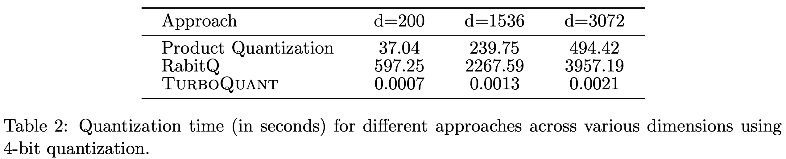
PQ requires running k-means to build its codebook is expensive and data-dependent. RabitQ is even slower and lacks GPU vectorization entirely. TurboQuant’s indexing time is effectively zero because the rotation matrix and codebook are precomputed once for the Gaussian distribution and reused for any input. No calibration, no k-means, no offline pass over the data.
This is what data-oblivious means in practice: the quantization time is essentially a constant, independent of dataset size or dimension.
7. Thoughts
The residual is the real innovation: The rotation and Lloyd-Max combination is elegant, but not entirely new; whereas Gaussianization before quantization has precedent. What genuinely surprised me is the residual treatment. Using a geometrically orthogonal tool for the remainder rather than just refining the same approach is the kind of insight that feels obvious in hindsight but clearly wasn’t.
The field analogy scales: The more I think about the sign quantization argument, the more I think it generalizes beyond KV caches. Any setting where you need to preserve angular relationships between high-dimensional vectors under aggressive compression like retrieval, dense passage ranking, multimodal embeddings, etc. QJL feels like a natural fit. I’d be curious to see it applied there.
m is an underappreciated hyperparameter: The number of random projections m is presented as a tunable knob, but the paper doesn’t give strong guidance on how to set it in practice relative to context length, model size, or task type. My intuition says this will matter a lot in production and deserves its own ablation.
No calibration data is both a strength and a question: TurboQuant’s Gaussianization guarantee holds regardless of input distribution, which makes it robust and calibration-free. But I wonder whether, for a known fixed deployment domain; say, a model exclusively serving legal documents, a domain-calibrated codebook would outperform the universal Gaussian one. The universality is a feature until it isn’t.
The backward pass is untouched: Like BitNetV2, TurboQuant focuses entirely on inference-time compression. The training loop is conventional. I’d be curious whether a version of QJL could be made differentiable, perhaps along the lines of DGEs from the FP4 training paper and used during training itself to close the train-inference gap further.
Orthogonality as a design principle: The deepest lesson here isn’t specific to quantization. It’s that when you have a budget of N bits, spending them all on one geometric tool is almost never optimal. Splitting your budget across tools that operate in orthogonal spaces like Cartesian MSE and inner product space here consistently outperforms going deeper on any single approach. That feels like a broadly applicable principle worth remembering.
8. Conclusion
At its core, TurboQuant is answering a question that the weight quantization literature never had to ask: what does it mean to compress something that is moving?
Model weights are static. You compress them once, offline, with all the time in the world to study their distribution and design the right codebook. The KV cache is the opposite as it grows with every token, shifts with every input, and must be compressed and decompressed at inference speed, token by token, with no opportunity to stop and recalibrate. The tools that work beautifully for one simply don’t transfer to the other.
We started this article by situating TurboQuant in the broader quantization story we’ve been building together. From the basics of mantissa and exponent in the FP4 article, to the extremes of ternary weights in BitNet, the thread running through all of it has been the same tension: fewer bits means less memory and faster compute, but also less resolution and more information loss. Every paper in this space is negotiating that tradeoff in a slightly different way.
What TurboQuant does differently is refuse to treat quantization as a fixed engineering decision and instead frame it as a constrained optimization problem with a clear objective which is to preserve inner products while minimizing representation bits. From that framing, everything else follows naturally. The rotation step emerges because you need a known distribution before you can design an optimal codebook. The Lloyd-Max codebook emerges because it’s the provably optimal quantizer for that known distribution. And QJL on the residual emerges because the last bit you have is worth more in a geometrically orthogonal space than it is refining a grid that already captured most of the structure.
Whether TurboQuant becomes the standard approach for KV cache compression or gets superseded by something better, the underlying principle feels durable: when you have a fixed bit budget, spend it across orthogonal geometric tools rather than going deeper on any single one. That lesson extends well beyond quantization.
With this, we come to the end of what turned out to be a genuinely long journey through some beautiful mathematics. As always, I’ve omitted nuances and simplified arguments to keep things readable, I’d strongly encourage going through the paper directly for the full theoretical treatment.
TurboQuant paper : https://arxiv.org/pdf/2504.19874
QJL paper : https://arxiv.org/pdf/2406.03482
That's all for today. Follow me on LinkedIn and Substack for more such posts and recommendations, till then happy Learning. Bye 👋