
Grokking model fine-tuning : A primer on fine-tuning methods
This article attempts to lay foundation for understanding the knitty-gritty details behind model fine-tuning and extending potential research direction in the area based on the learnt principles.


In our previous article, we discussed about language shared subspaces and usage of fine-tuning to work with downstream tasks. Though we discussed at length over spaces and representations, the fine-tuning aspect was left as black box to be cleared out in future articles.
Table of content
Introduction
Ideal case / need for fine-tuning
Why does fine-tuning work?
How does fine-tuning work?
Methods to fine-tune
Dreambooth
Textual inversion
LoRA
IA3
Hyper-Network
Method comparison and conclusion
What we learnt today?
Introduction
Representation form the core of all the significant developments in deep learning. Be it any modality, example, images, text, speech, etc. a high quality representation is always the basis of the downstream task.
We had been discussing the importance of representation in multiple previous articles


With efficient architecture choices and huge amount of compute and available data, larger and larger models are trained and published which are capable of high quality representations. But, these training are often time consuming (as they are done at scale) and compute intensive. Though these models are able to learn /explore a large section of manifold, they miss the pinch of specialization needed for most downstream tasks.
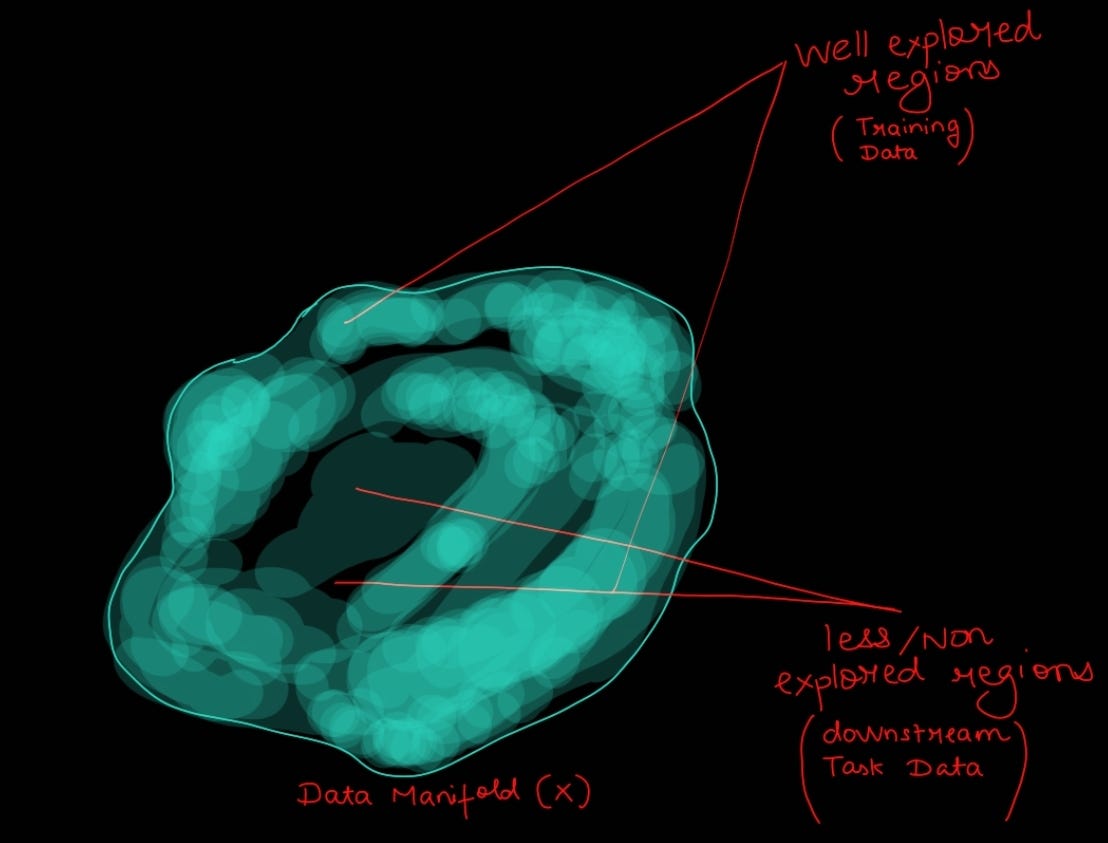
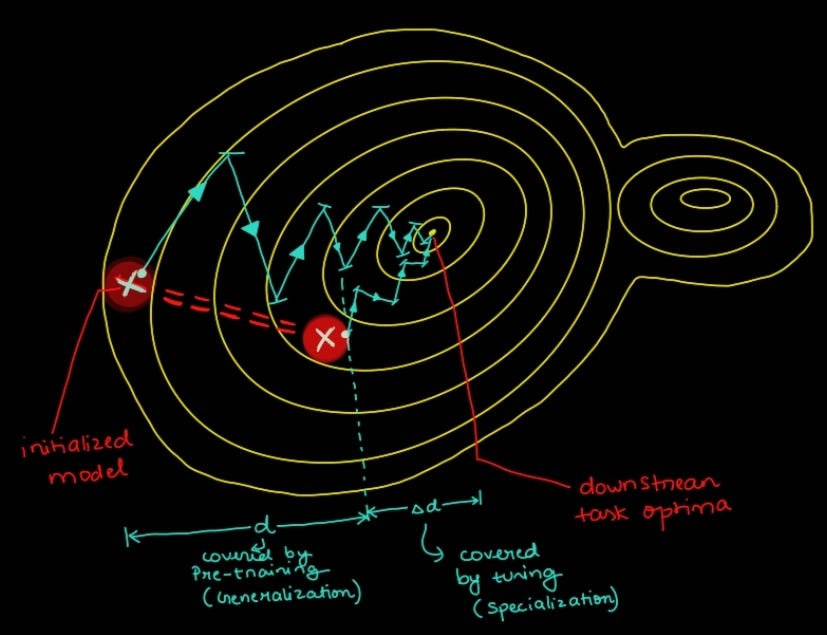
Hence, we want want to go from generalization to specialization. The simplest way would be to train the model from scratch. But, imagine re-exploring the entire manifold/data surface and still learning a sub-optimal space. This not only wastes compute and time, but, also the model is very sensitive to noise (check out regularization article to understand why this happens).

Next intuitive step is to reuse the existing model and re-train on our data. This would ensure that we are already starting from a well explored region and then focussing on certain area.
Ideal Case / Need for tuning
1. We have large, well trained models capable of generating high quality representation.
2. Training these models from scratch is slow and cumbersome. It also requires large number of datapoints as significant amount of parameters have to be updated.
3. We want to leverage pre-trained model for specializing on our downstream task.
4. The method to do so, should be data and compute efficient and robust.
This is where fine-tuning walks into the picture. But, what is fine-tuning? And why does it work?
Why does fine-tuning work?
As inferred from above discussion, simply put, it is a method to refine your Pre-trained model over a specific task to make it more specialised with much smaller dataset sample. For a visual narration, you can think it like this:
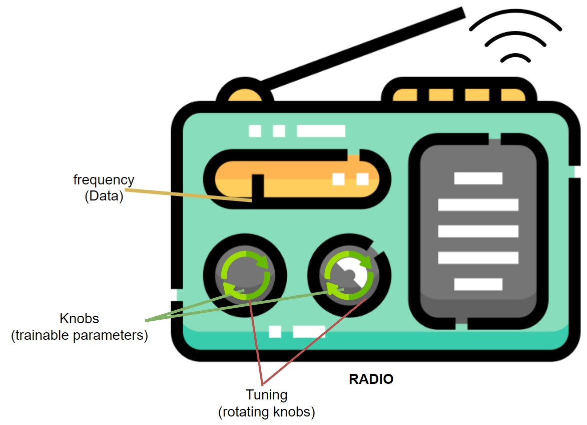
Imagine a radio, it has bands for all frequencies, to listen to a certain channel, you have to adjust the knobs while hearing the outputs in form of sound/music. Here, radio is your model, set of all frequencies is data, knobs are trainable parameters, adjustment of knob signifies tuning/parameter updates and listening is your supervision through which you calculate delta (Δ).
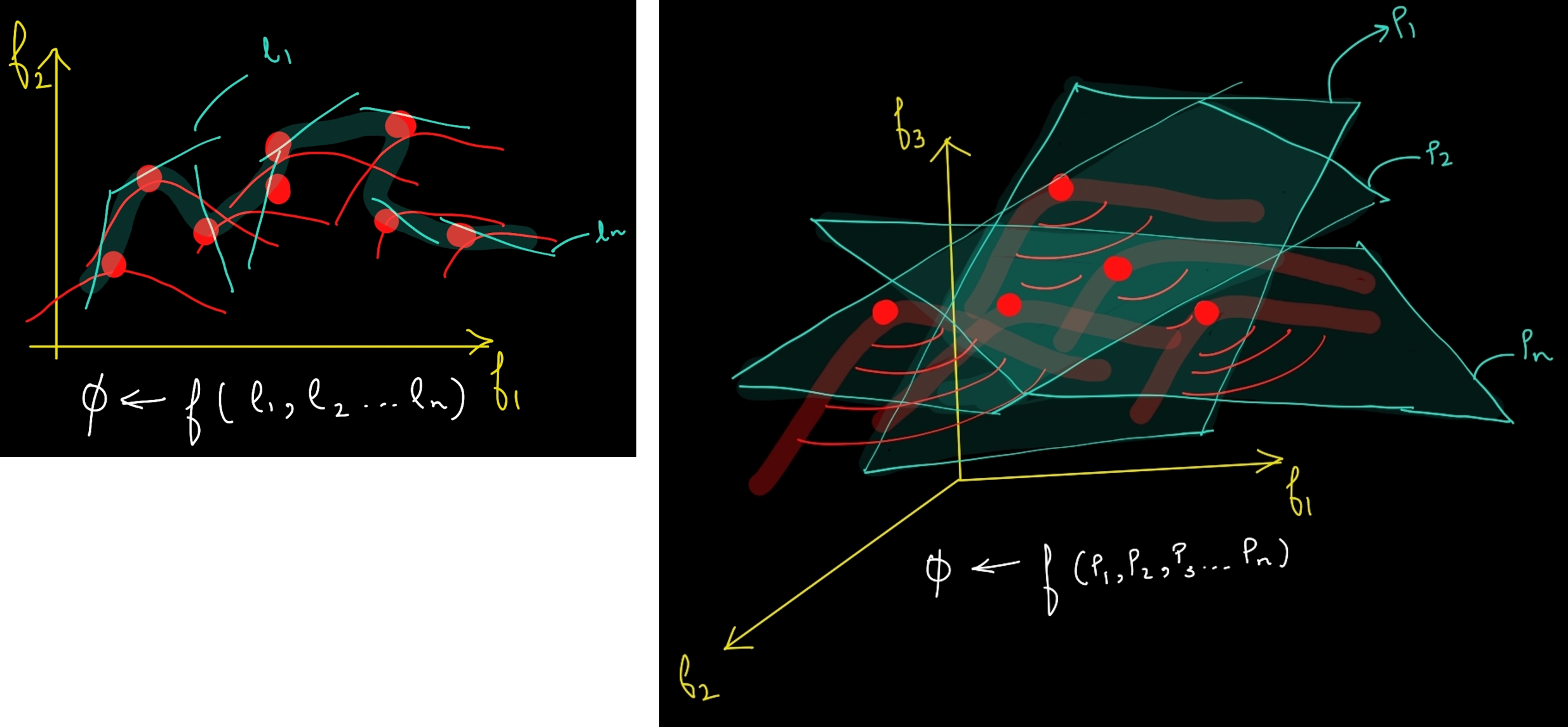
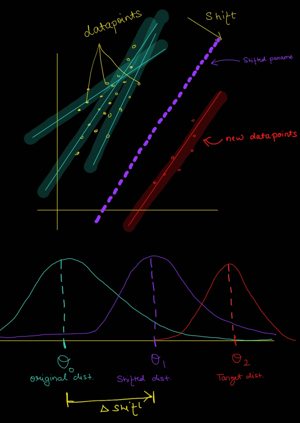
To understand it more clearly, let’s take the below mentioned diagram into perspective, the red points are data points and red curves are fitted polynomials on top of them, whereas the blue lines/planes are output /solution space, each of these polynomials are parameterized and hence trainable. Lets say you added N new points and we want to accommodate them into our model, for sure we don’t want to shift and scale all these lines/curves as it would lead to such a drastic change in weight/param that the model forgets the previously data distribution, maybe few of them could be fine. Hence, we just selectively parameterize them and tune, this results into shifting/scaling of our solution plane as well as underlying curve/parameter space.
Thanks to our discussion till here, we now know why? of fine-tuning, let's dive deeper into how? of fine-tuning. The entire idea lies somewhere between Self-supervised learning and Semi-supervised learning.
How does fine-tuning work?
Arguably, there are two ways to tune any model (each method have its own intricacies to develop more variations, but, underlying assumptions are derivative). They are as follows:
Tuning by freezing : Here a model trained on very large dataset either through Self-supervised learning or supervised learning is taken and freezed. This serves as backbone for feature extraction/representation generation. This representation is then just navigated to the required task by another network/small model composed of few layers. This smaller model is easy to train and also has a simpler task to conduct (assume), hence, it saves lots of compute and time, while giving good quality results. But, the underlying assumption behind this technique is that the smaller model will be able to project the current representation in a expected output space, which might be tricky depending on complexity of projection layer of feature extractor/backbone. Hence, often times this fails to deliver good quality results.
Tuning by controlled gradient update : This involves training of entire model, but, instead of using full gradients; they are scaled down by a factor, to prevent corruption/over-specialization of representation space. Though this gives good quality outputs, but, is susceptible to catastrophic forgetting. It is also difficult to control as there are additional hyperparameters for gradient strength and yes, the training itself is compute intensive and slow.
Every tuning method is/tends to be composition of these two methods. Now the question is we know how to tune, but, what to tune?
Quite simply we can just say model, but, profoundly, we can tune anything that is parameterized. It could be model, it could be sub-section of model or it could be an additional set of vectors not part of model, but, signifying/representing the data. This idea could be represented by the image below.
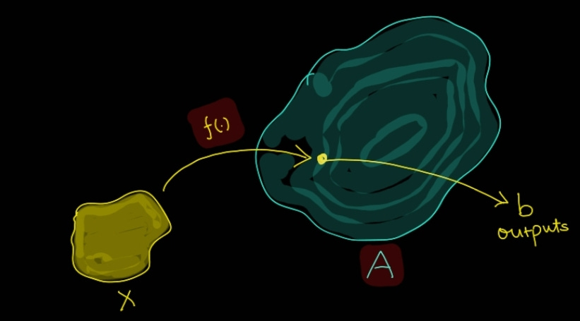
A in the above image could be viewed as your model, x is your datapoint, b is the output and f is the transformation of data to model space. You can either tune A (in this case f(.) will be Identity) or some representation of x itself (completely isolated from model) which basically is f. We will discuss this more in-depth in later section.
Consider this example for better understanding, you have two variables a and b and your task is to add them to get a number c, you can then either change a or b to reach your objective.
All of this now known, lets now explore common tuning techniques and their intricacies. We will also connect each of the techniques to corresponding idea we discussed above.
Methods to fine-tune
Before exploring each method one by one, let's get our requirements straight,
A compute and sample size friendly method, but, should also be easier to control (either in supervised, or Self-supervised way)
Less prone to catastrophic forgetting (which as the name suggest is the change in manifold of weights such that it leads to noising of all prior info)
The process to do this, should scale and hence be agnostic to a model type, hence, the method should be a plug-and-play in nature.
Keeping these requirements in mind, let's move onto the methods to realize our requirements (we will be looking at each method from text2image generation diffusion models perspective as it is easier to explain, the explanation could be extended to any modeling choice. Also, we won't discuss on the implementation/data preparation side of things much).
Data preparation
Datapoint is represented in form of (image, text pairs).
The text component is any unique identifier, example XYZ. The sole purpose is to have a non semantic disturbing identity. Imagine you put the identifier as "blob", this would seemingly disturb models knowledge on blob.
The text looks something like "A photo of XYZ", "XYZ eating pancake", followed by image with object/subject in action.
Fine-tuning method discussion
Dreambooth
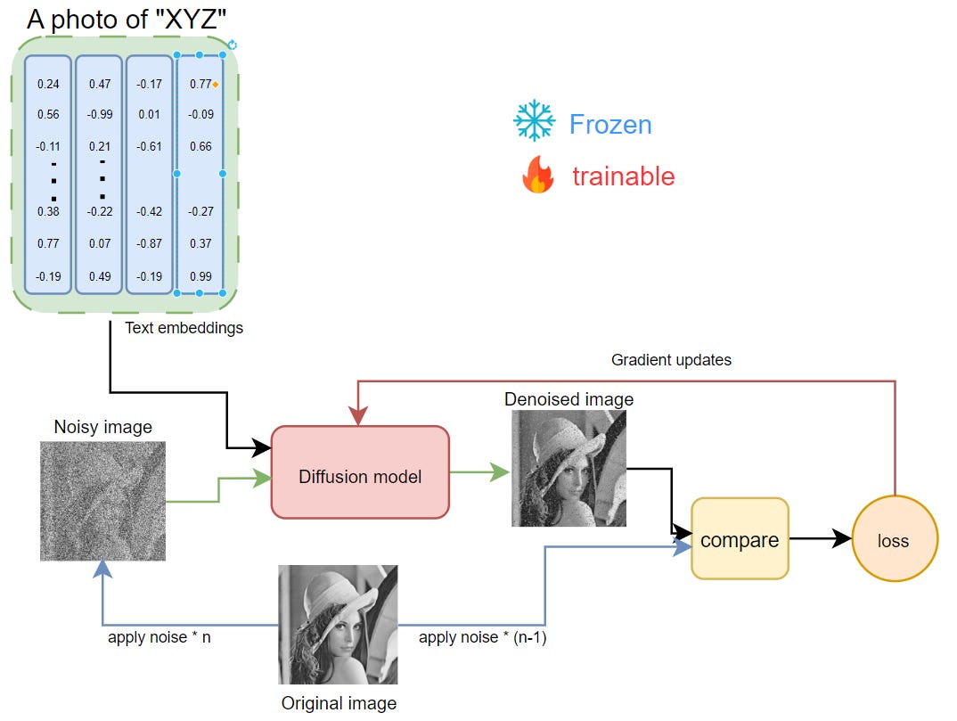
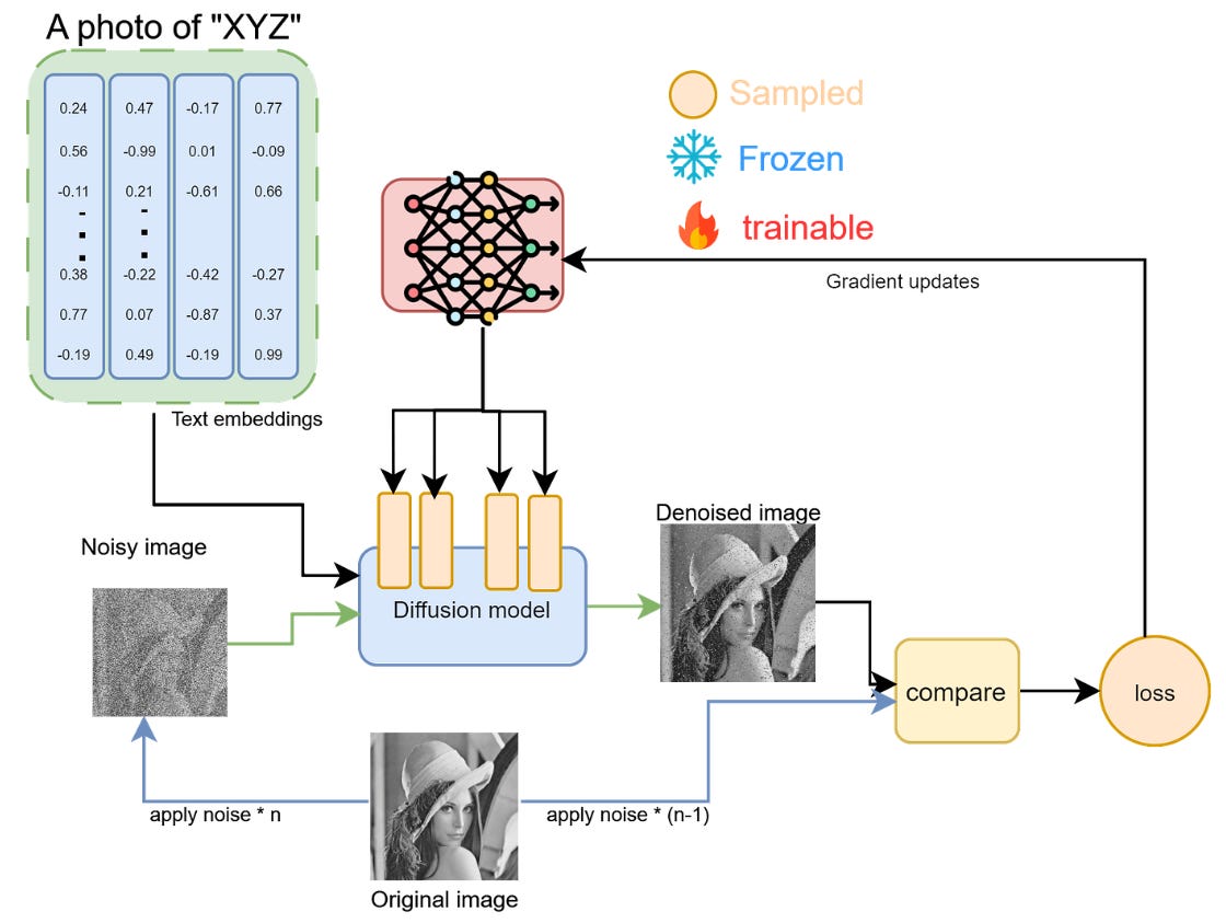
Dreambooth tuning process Dreambooth is possibly the simplest method as it directly updates the entire model. It requires full scale model tuning, hence, huge amount of compute and data is required. Given its inefficient tuning paradigm, it's difficult to scale across multiple use-cases, but, the generated samples are of really high quality and tends to be more strongly aligned to the text/prompt.
Methodology
The input text is converted into embeddings and corresponding image/sample is noised.
This is then fed into diffusion model for refinement along with text embeddings.
Then the model iteratively denoises the corrupted/noisy image, which is then compared against the ideal one for every step t.
This comparison gives us the accumulated loss, which is then back-propagated to the diffusion model to calculate gradients. These gradients are then used to update the weights by chosen optimizers.
By doing this model learns to align a given text identifier and image pair together, and as it is trained on huge set of images, is able to form correlation between the learn representation and the new datapoint.
After tuning, model might face forgetting and for each new case we will end up with a newer model (though the capacity of such method is huge, as we are using full parameter space) of full size, example, 5gb.
Advantages
High quality representations and hence generation.
Easy to setup and tune.
Disadvantages
slow, heavy dependency on data size.
larger compute required, and hence difficult to scale.
Textual inversion

Textual inversion tuning process In the How? Section of our discussion we saw that either model (A) could be tuned or some representation of inputs/text (f) could be tuned. Textual inversion follows the latter, instead of tuning the entire model, which leads to huge amount of weights for every single task, why not just learn a representation such that when this gets projected to model space; is able to take us to the expected representation region. This would mean that for every object we would have a unique key/embedding, which might not make sense to us, but, actually is an approximate mapping to the expected output space.
Methodology
We parameterize the previously fixed embedding space for the unique identifier "XYZ", hence, the computed gradients could be accumulated on top of this embedding. The diffusion model is frozen completely.
The remaining process remains same, but, the gradients computed is flown all the way back to the embedding to update it such that the projection of this embedding onto model space leads it to the region from where model can give a high quality output representation/denoised image.
This method though is fast to tune and even scales well, suffers a huge setback because of its assumption over models capability of projection which is dependent over the quality of learnt embedding. As the parameter space is very small, the method is not able to learn a verbose enough representation and hence fails to deliver high quality outputs.
As for the inference, let's say you have 10 objects/subjects, each of them will have a set of associated key/embeddings. These embeddings are much smaller in size (few kbs to few mbs), hence, for any specific generation of a subject doing something, the corresponding embedding is simply fetched and projected onto diffusion model for generating image.

conventional adverasrial attack The method would seem very familiar to adversarial attacks(read about deepdream) on images, as even there we compute the smallest delta required to corrupt image (without changing/affecting the model) in such a way that it's humanly impossible to determine any change, but, is able to confuse the model.
Advantages
faster convergence and less compute requirement.
scalable and efficient handling
Disadvantages
weak representative power, hence, lower quality outputs/images.
LoRA (Low Rank Adaptation)

LoRA tuning process LoRA or Low Rank adaptation is probably the most commonly used choice for tuning large architecture. It falls under the family of PEFT methods (Parameter Efficient Fine Tuning). As the name suggests the algorithm in this family, employ techniques to tune large models at scale while changing/tuning a very small sample of parameters. LoRA is especially applied on attention blocks (which is simply a dense matrix).
MethodologyThe entire model is frozen including its attention layers, and it follow the same process flow as above methods (check image)
Our major plan is to tune these attention matrix (composed of KV correlation). For doing so; we simply attach another matrix of same size and then just tune it. The output from frozen and trained matrix could then be aggregated. But, the issue is that we want our method to be efficient, otherwise why don't we just do tuning of attention matrix directly. Hence, instead of a full rank matrix, we assume that new information corresponding to data in our dense attention matrix has much smaller rank, which then could be simulated by decomposing the dense matrix into two lower rank/smaller matrix.
This decomposed matrix could be imagined as an under-complete autoencoder with a very small bottleneck, also referred as adapters in LoRA terms. Check the diagram below for clarity. Only this autoencoder is tuned, but after completion of tuning, the original attention matrix and tuned/adapted low rank matrix are combined for inference.
The computed loss over the generated and expected image is used to only update the adapter weights while keeping all other model parameters frozen.
Advantages
LoRA is an efficient yet effective way to perform tuning at scale, as the adapters are much smaller in size and hold a lot of information as there task is to only learn the delta (Δ) between the current model capability and the expected one.
Given its ease of use and setup, it could be easily plugged and played with multiple other methods, example, you can use textual inversion and lora together.
No additional compute cost during Inference as the LoRA weights are merged with the frozen model weights after tuning,the model size is around 100-150mb.
Disadvantages
Heavy dependency on pre-trained/host model, as we know it's task is to learn the Δw component from (w+Δw), if base model is not well trained, LoRA being a low powered/rank architecture fails completely.
Task alignment becomes a issue, as LoRA fails in generalizing across multiple downstream tasks, but, eventually this also depends on host model to a larger extent.
Interestingly, LoRA is not a new concept at all, Low rank matrix approximation is a common and well researched topic. Also, the formulation used to define lora could be re-structured to calculate the exact weight required to accommodate new datapoint, which leads to very famous kalman filter as well (as kalman filter also performs low rank approx).
Check out the derivation in the image below.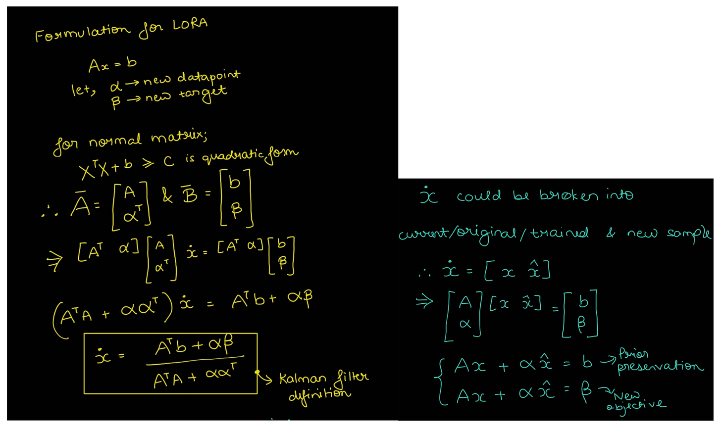
Low Rank approximation formulation with kalman filter as by-product


IA3 (Infused Adapter by Inhibiting and Amplifying Inner Activations)

IA3 tuning process This is a relatively newer method which stands for Infused Adapter by Inhibiting and Amplifying Inner Activations. As we saw in LoRA; we were trying to approximate the full rank attention matrix by a lower rank matrix, but, what if instead of using any matrix formulation we do it only with vectors as we did in Textual inversion (although we are not going to apply adapters on data).
Methodology
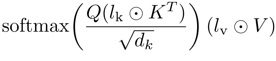
This method adds trainable parameters on top of activations in cross attention layers after softmax (in LoRA it is done before softmax as we are decomposing attention matrix itself), which for the key matrix is just
(Kx1)and for value is(Vx1); this is much less than LoRA, hence this matrix only rescales the outputs by updating the corresponding key and value matrix and thus leads much smaller adapter size.
These trainable adapters/vectors are attached onto the Key and Value matrix while tuning.
As it is part of model itself (similar to LoRA) but only work as scaling mechanism (similar to textual inversion), it falls in sweet spot between both.
The tuning and inference process remains exactly same as that of LoRA.
formulation for scaling term in IA3
AdvantagesFaster and smaller in adapter size against LoRA (less than 1 mb).
Disadvantages
It shares similar tradeoffs against full fine-tuning like LoRA.
Representation power again becomes a question as in Textual inversion, though it has more supporting parameters attached now.
Hyper-Networks

HyperNetwork tuning process They are unpopular yet interesting methods to tune a model. It is seemingly inspired from meta learning framework, where instead of tuning a certain network itself, we use a driver network to learn a distribution from which the sub-network could be sampled. Imagine a parent neural network giving parameters for another network.
This could more strongly align with variational Inference, where we assume another function (here Hyper-network) to learn an unknown and harder to sample distribution (here Lora adapters). You can imagine LoRA as a single point estimate (as it learns a single set of parameters after fine-tuning). Now imagine using a network to optimize the adapters to learn the representation in continuous space by sampling.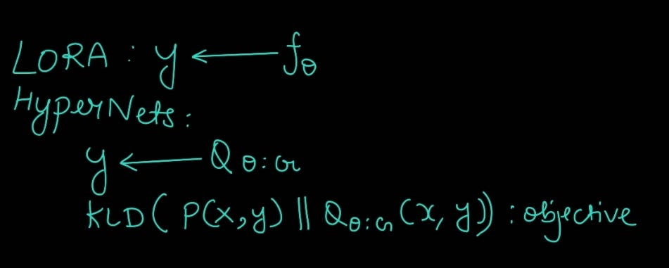
HyperNets formulation against LoRA Methodology
Instead of updating LORA through gradients being derived from a defined loss function (simple and prone to our constraints on metrics), we use Hyper-network as selector/sampler and updater, while the Hyper-network itself is updated by defined loss. It's like optimizing a single equation vs optimizing multiple and choosing the best one.
The tuning process is similar to above ones, the only difference is that instead of adapters getting their updates from computed gradients, here, the adapters are updated through Hyper-network which in itself is updated through the actual gradient update (check image for more clarity).
AdvantagesSmaller adapter size than LoRA.
Usable output quality.
Disadvantages
This optimization requires search in Hyper-network space and hence for more data-points are required for effective exploration.
Slow (takes a lot of time) and difficult to optimize.


Method comparison and conclusion

From the entire discussion and summarization from above table we can conclude;
Fine-tuning is not a scalable solution but is really descriptive.
Textual inversion is fast and scalable but doesn't generate high quality outputs.
LoRA is a preferred choice along with IA3, as not only they are fast to tune but also, the adapters are very small in size, hence, multiple adapters could be readily tuned and stored, eventually they could be loaded and off-loaded selectively based on use-case.
Hyper-network are interesting but not quite there yet.
So, overall winner is PEFT family, i.e. LoRA and IA3.
What we learnt today?
We understood What? Why? And how? of fine-tuning and we dived deeper into the reasons why fine-tuning works.
We came up with an objective for ideal situation to all our fine-tuning tasks.
Then we discussed each fine-tuning method which included Dreambooth, Textual inversion, LoRA, IA3 and Hyper-network in reference to image generation using diffusion models and learnt the working, advantages and disadvantages behind each method.
Finally, we concluded our findings and learnt that LoRA and IA3 (PeFT) are preferred methods to perform task specific fine-tuning.
That's all for today.
We will be back with more useful articles, till then happy Learning. Bye👋