Large Concept models : Language Modeling in a Sentence Representation Space

Re-imagining the core principles behind representation generation in foundation model.

In our previous article Byte Latent Transformer :

Byte Latent Transformers : Patches Scale Better Than Tokens

We understood the issues with current tokenization methods and available methods to overcome them. We saw how we played with the pre-processing and encoding block to make a robust and efficient architecture to use at scale. The decoder in BLT also followed the same paradigm. The only thing we kept generic was the central processing block (which was a simple transformer architecture, with slight changes, but the core mechanism remained same).
This article follows the work on and around the processing block in a recent paper from Meta called as Large Concept models, we will discuss the methodology, outcome and underlying algorithm/thoughts behind it. But, before that, let's make a quick diversion for setting up the context.

concepts are latent/hidden

---

Table of contents

1. Overview of induced biasness (Biasness: The good, the bad and the ugly)

2. Core objective

3. Methodology

   1. Model overview

   2. Data pre-processing

   3. Metric for evaluation

4. Architecture deepdive

   1. Encoder module (SONAR encoder)

   2. LCM

      1. Base LCM

      2. Diffusion model LCM (one tower and two tower)

      3. Quantized LCM

   3. SONAR brief overview

5. Outcome

6. Thoughts

7. What we learnt today

---

Biasness: The good, the bad and the ugly

We discussed in BLT article that any sort of inductive biasness leads to restrictions in terms of representation, but, biasness could be helpful in cases where criterions are well known and defined. Hence, any assumption would not omit any feature or required correlation. The underlying biasness limits the number of parameters we have to deal with hence preserving precious resources and time, being robust and efficient at the same time. For example, imagine fitting a sine curve, you either carefully design the activation and parameter space or define a model with huge set of parameters hoping that it would learn the curve eventually. Physics informed neural networks actively use these inductive biasness for defining boundary conditions. One of advantage it provides is interpretability, as the boundary conditions are known you can efficiently interact with much less / range restricted features and interpret results. In one of my post here

Regularization : What? Why? and How? (Part -1)

I mentioned how these restrictions/biasness/regularisation effects number of parameters and the shape of surface on which entire optimization is happening. From here on, we will mostly talk in terms of shape on space/manifold for better understanding.
Hence, in summary,

• The good, Quality restrictions/biasness provides options for robustness, interpretability and efficiency.

• The bad, the space where we are applying the constraints are supposed to be known and defined.

• The ugly, ill defined biasness leads to poisoning in data understanding and hence in approximation.

metric hard to define in pixel space, easier in embedding/information space

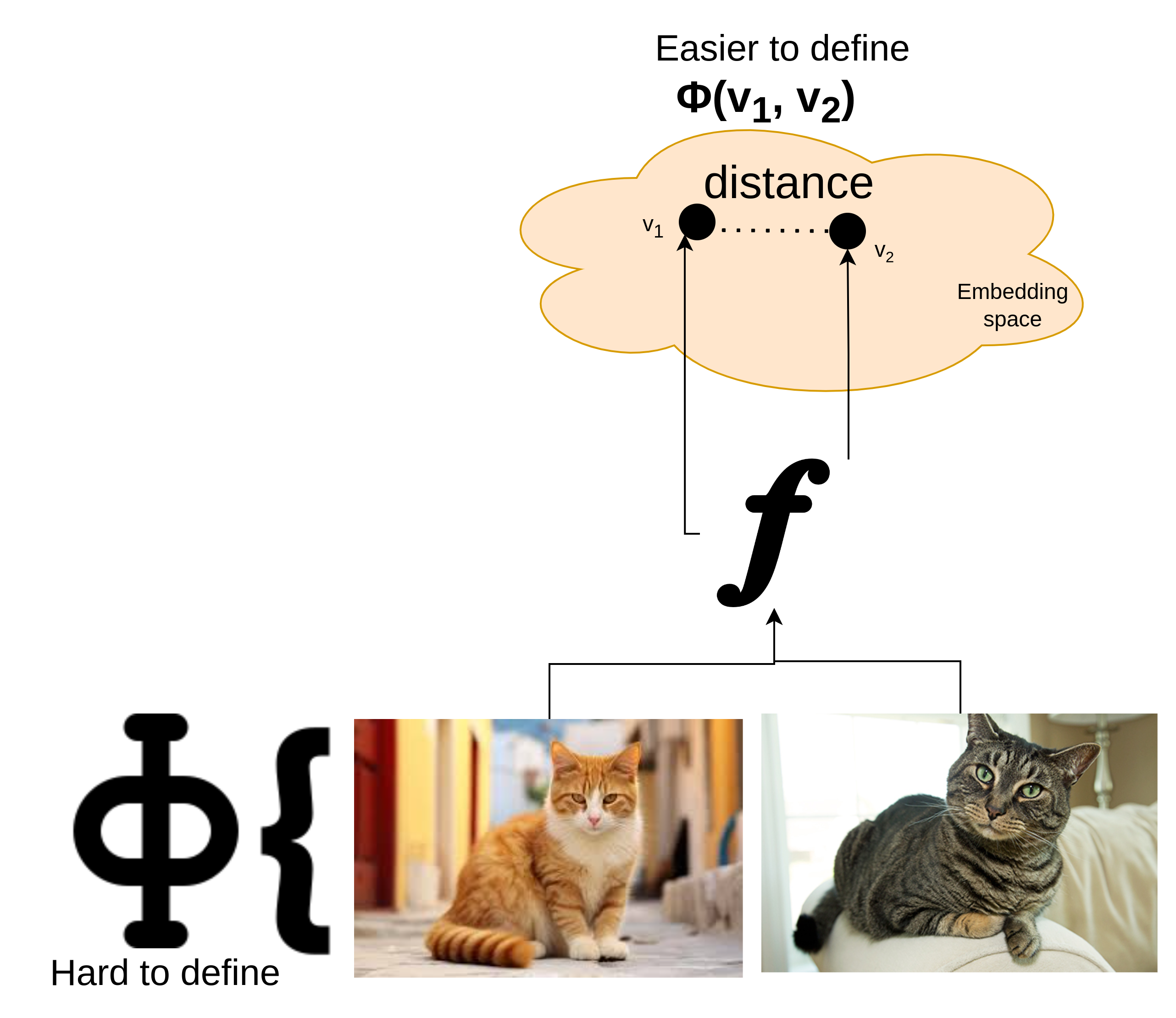
Something to note here is that we never have any known or wide enough boundaries for data itself, for example, how to parse text? How to combine tokens? How to add two sentences? How to add two images? Hence, the operations on top of data itself is challenging. This is typically a contextual and semantic tasks, which could only be done in some abstracted out space, where we only have representations. These representations/embeddings capture the essence of data, which we can call as information. The information typically lies in much lower sub-space (imagine, a cube as your data and two opposite diagonal lines as information, you can retrieve the cube back if given these lines). But, it is easy to figure out this information space for cube and then perform computation on it (where we know the structure) what about the non-conventional data points (like an image, text)? We need a function that takes in data and gives out a compressed version of it and then we need to perform specialized operations on top. We can make simplistic assumption over the shape and nature of space, hence can define our metrics.

similarity2 metric is easier to understand and define as it is applied on embedding/concept space.

Now, we have two things in hand,

1. An encoding function to bring in data to a certain space where we can perform operations.

2. An Operation/processing function to efficiently perform operations on the lower dimensional information space.

The encoding function, could be referred as Kernel function can be anything (as we saw in BLT) or as in the LCM paper called as SONAR (we will discuss this later)

What about processing function? It could be anything, we can define it as a generic one, which means we can put in our biasness on shape of manifold, we can make it as a single-step transformer, a torus or put our assumption over how we move on the manifold as in diffusion models. Hence, we are not applying biasness on the data, but on concepts, and that too on how we explore concept space and its shape.
To concentrate only on operation/processing, we can just fix the encoder block (containing a sufficiently good tokenization strategy and encoding mechanism, hence SONAR used here) and only work with processor, such that, our only task becomes learning the operations in sub-manifold without ever worrying about learning the encoding/decoding.

---

Core objective

moving in concept manifold for task summarization

1. Isolating the representation and computation block to separate tasks and operations (tasks like language modelling, representation of modalities, etc. and operations like projection, addition, etc.)

2. Learn a general framework over the representations/concept which is not inherently data dependent, you can imagine how powerful the framework becomes (as you can make assumption over what shape would it be as well as how you move on the shape).

3. The processing framework should be able to map from input-embedding space to output-embedding space (which could then be handled by a fixed module, i.e the encoder-decoder module).

4. In paper, the authors didn't much work on the shape of the manifold (though that is a strong possibility), the pivot of the work is diffusion model (how you move on the manifold) at core for information process (which we will discuss in later section).

   ---

Methodology

Model Overview

Core architecture

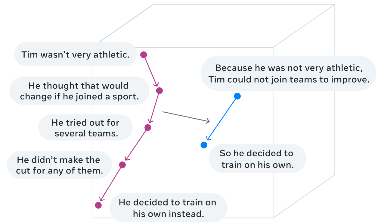
The LCM operates in sentence representation state, which means it takes in current sentence as input, encode->process->decode it to next sentence, other/generic architectures do this at token level.
To put this more firmly, generally for any decoder only models (gpt series), the objective is next token prediction, hence, it generates token by token in sequence. The LCM architecture (which includes encoder-LCM-decoder modules) objective is to predict next sentence directly given previous one. This specifically means that sentence are the smallest unit for information in LCM.

step by step process

let's have a quick walkthrough of the architecture first.

imagine the grid as latent/embedding space, nodes as projected concepts and edges as relations and connections, by learning the concept-to-concept regression we are basically exploring a high-dimension graph

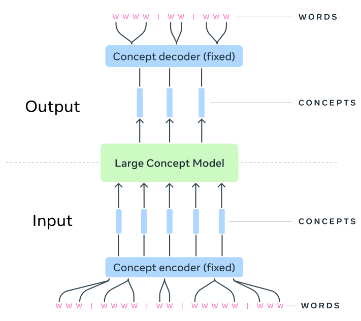
1. Data to concept : A Module translates from modality to concept (in form of representation), hence, it's a words/modality to Concept module (basically a encoder)

2. Concept to concept : This is primary LCM block, it performs operations on represented concepts.

3. Concept to task/modality : This converts concept/representation to modality back.

   

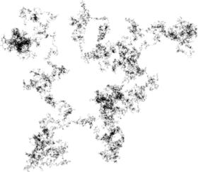
   (hypothetical) latent space after concept-concept regression, dense regions are concept clusters

Data Preprocessing

1. Segmentation:

   • Data is segmented into paragraphs using the Segment Any Text API.

   • Paragraphs are constrained to a maximum of 10 sentences, merging smaller consecutive paragraphs where necessary.

2. Plan Concepts:

   • Synthetic high-level topic descriptions are generated for each paragraph using the Llama-3.1-8B-IT model, which balances topic quality and generation speed.

   • Approximately 320M paragraphs (1.5B concepts or 30B tokens) are processed.

Metrics for Evaluation

For pre-training evaluations multiple metrics are taken into account like l2 distance, contrastive accuracy (The ratio of embeddings in a batch that are further away from the predicted embedding than the ground truth), paraphrasing (semantic metric/cosine similarity between generated and context embedding, i.e last k sentence embeddings) and mutual information (difference in unconditioned and prompt-conditioned perplexity scores) is used.

---

Architecture deepdive

1. Encoder module : This is fixed block which is composed of SONAR ( a Pre-trained encoder-decoder foundation model) which takes in sentence as input, performs character level tokenization and encodes it in into an embedding. But, why character level? It's mostly because of experiment design to prove the LCM block is the determining factor in performance. Obviously we can set methods like BLT for better representation.

2. LCM module : This module auto-regressively predicts the next sentence concept/embedding of next sentence given previous concepts. As this is operating solely on concept-to-concept basis; it inherently is language and modality agnostic. As I mentioned that now we have an isolated block, we have a huge degree of freedom over how we design it's surface or how we move on the learnt manifold. Taking that into consideration, paper tried out three distinct methods.

   1. Base LCM
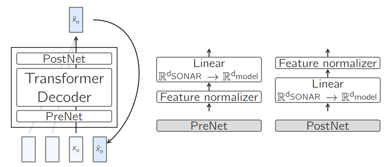
      Simple transformer based architecture, MSE serves as objective for embedding/concept alignment. It has a simple modelling choice, yet, works with zero-shot baseline tasks. The base LCM module has three distinct sub-modules (A PreNet, a decoder block and a PostNet):

      

      1. PreNet : This serves as pre-processing block, which normalizes the input SONAR embeddings and maps them to the model’s hidden dimension.

         \(PreNet(x) = normalize(x)Wt_{pre} + b_{pre}\)

      2. PostNet : Its exact opposite of PreNet; hence denormalized embedding and maps it back from models hidden dimension top SONAR space.

         \(PostNet(x) = denormalize(x)Wt_{post} + b_{post}\)

   2. Diffusion based LCM
      As the name suggest, it is inspired by diffusion models, conceptually, assume your embedding of current sentence as e_t, you iteratively add noise to interpolate to the next sentence embedding e_t+1, models task is to predict this added noise iteratively to remove during backward pass and hence get the sentence concept.
      Simply put, during backward pass, for any step t, we denoise a random state embedding conditioned with previously cleaned sentence embedding iteratively to get next concept. There are multiple flavors to this process, in LCM paper the authors predicted transition from e_t to e_0 (similar to Latent consistency model paper¹) instead of sentence-sentence transition. Hence, during inference, you start from e_0 remove noise t times to get concept embedding at t.

      

      A typical diffusion process, red/orange region high energy (bad samples/noise), the blue regions are low energy regions (data samples)

      As the model learns the interpolation itself, hence has a better understanding of concept manifold. You can imagine this like directed walk in space from point A to point B, which if retraced; takes you back to A. But, in the process, you end of exploring the non-important space and hence learn the manifold, check the diagram for clearer understanding. (The rabbit hole is much deeper here, we can discuss about Energy based models, random walk in higher dimensions, and much more, but, let's leave it for future blogs).

      The authors experimented with two different architectures for forward and backward pass:

      

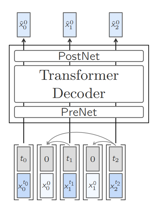
      Training of One-Tower diffusion LCM. Interleaving the clean and noisy embeddings and sampling different diffusion timesteps allows for efficient training.

      1. One-Tower Diffusion LCM: This is standard architecture where the Autoregressive forward and backward pass is done through single backbone/Base-LCM block. For efficient training, the model is trained to predict each and every sentence/embedding in a document at once which is done through interleaved clean and noisy embeddings, hence for each embedding at time t, we have a noisy embedding at t (in dark blue) and cleaned embedding (in light blue) which could be concatenated and trained in one-pass.

         

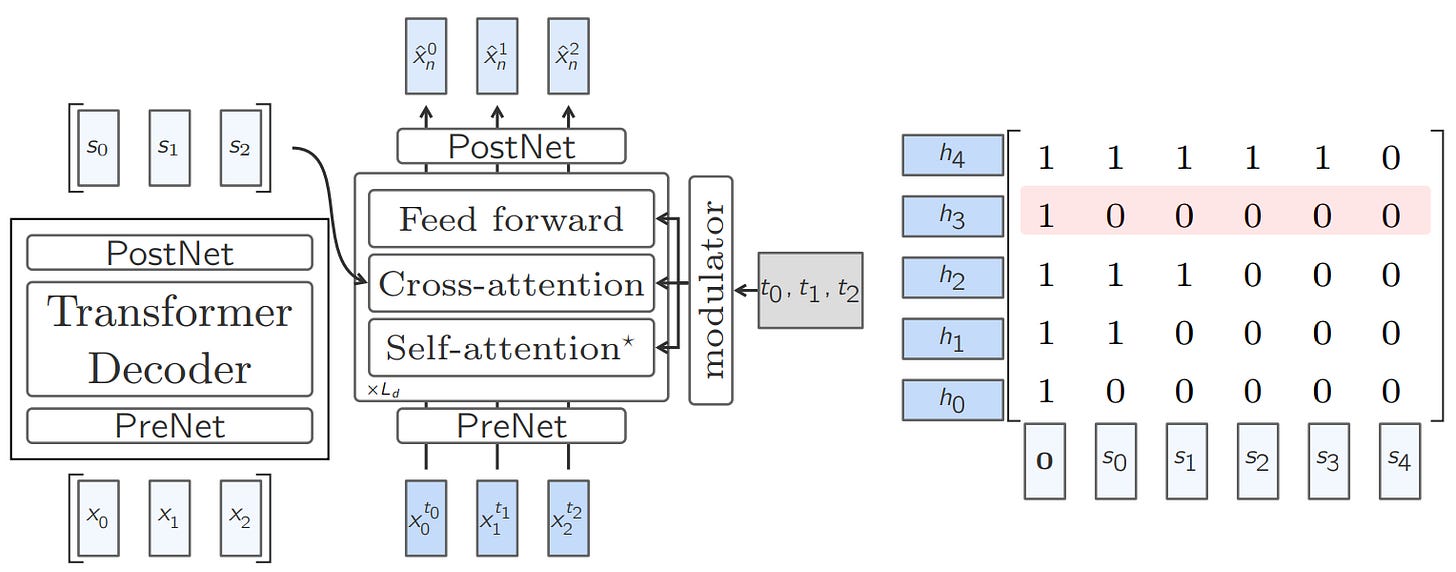
      2. Two-Tower Diffusion LCM: Here the architecture is composed of two blocks, first, a contextualizer; which simply is a decoder-only Transformer with causal self-attention. The outputs of the contextualizer are then fed to a second model called as denoiser, which iteratively denoises the embedding to predict clean concept level embedding. Denoiser is composed of cross-attention block to attend encoded representations from contextualizer.

         

   3. Quantized LCM
      The key idea is residual vector quantization for efficient representation. They follow a method similar to VQ (vector quantized) models, but following the methodology of diffusion process we discussed (discrete instead of continuous). Basically, your sentence embedding from SONAR is mapped to a pre-stored codebook RVQ (a dictionary of residual vectors retrieved by discrete representation of SONAR), the closest representation serves as next state, which is then refined over multiple iterations using the multiple codebook lookups. This method is efficient as instead of moving onto a continuous space you are in discrete space. RVQ is simply a set of vectors representing a concept where each vector represents remaining information left after previous vector/representation. Its similar to how we have a group of eigen vectors representing a matrix, where each eigenvector info/importance defined by eigenvalue. Eigen vector 1 is formed out of majority info, the next largest is formed over the remaining info.

      

      M = A+B+C (here A is matrix from largest (majority info), B from 2nd largest and C from smallest eigenvalue and corresponding vector)

      For simpler example, imagine a greedy world where a person A has 5 chocolates, someone comes and takes 3, the next person cannot take more than first and hence takes residual/remaining ones.

      

      That said, lets see how each of the ideas faired out, empirically,

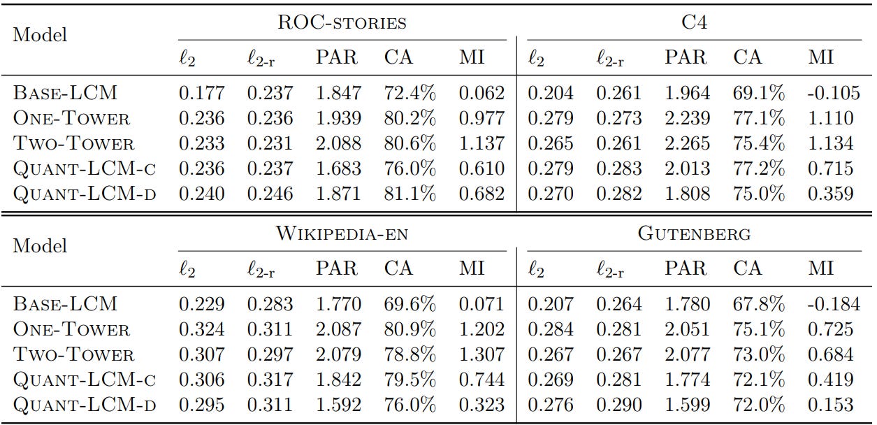
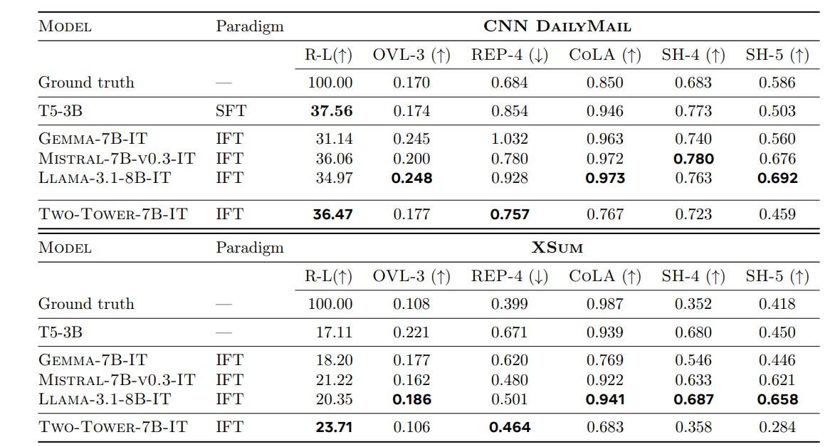
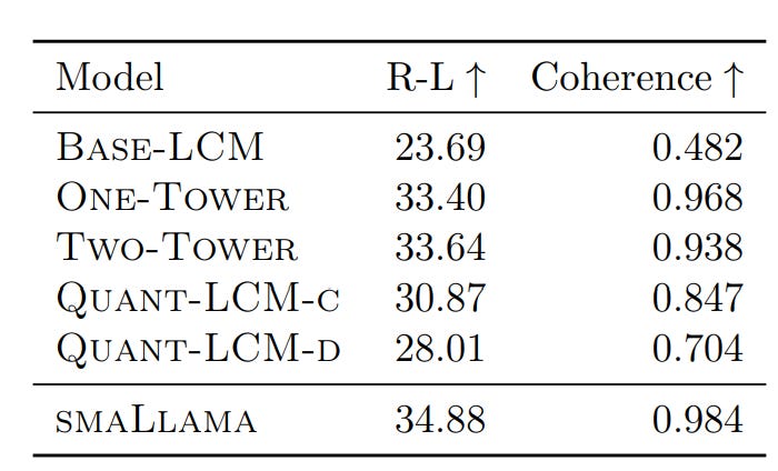
      1. Diffusion-LCM and Quant-LCM variants show similar ℓ2 and ℓ2-r scores, despite differing learning objectives.

      2. The Base-LCM has the lowest ℓ2 score (expected due to its training objective), but it does not improve ℓ2-r scores compared to other models. Base-LCM generates an average of plausible continuations in SONAR space, which may not correspond to relevant points, leading to poor performance on CA and MI metrics

      3. No significant differences in CA scores between Diffusion-LCMs and Quant-LCM variants. MI scores are Higher for diffusion-based models due to better paraphrasing of context. Quant-LCM significantly outperforms Base-LCM.

      4. Quant-LCM Variants: Quant-LCM-c outperforms Quant-LCM-d, likely because predicting codebook indices with cross-entropy loss is harder than using an MSE objective.

      5. Diffusion-LCM Variants: No consistent difference between One-Tower and Two-Tower diffusion models across metrics and datasets. In overall, diffusion-based methods perform best for next-sentence prediction in SONAR space.

         

         comparison of different modeling choices

3. Decoder module : The regressed sentence-level concept is then decoded back to output space, which could be text, audio or other modalities. The decoder block is part of SONAR architecture.

4. SONAR overview

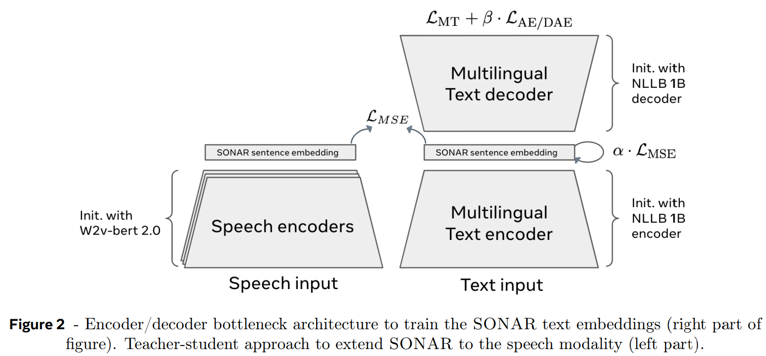
   It was first introduced here, which served as fixed size embedding space for multilingual and multimodal inputs. It covers 200 languages for text and 30+ languages for speech. A brief summary of the SONAR:

   

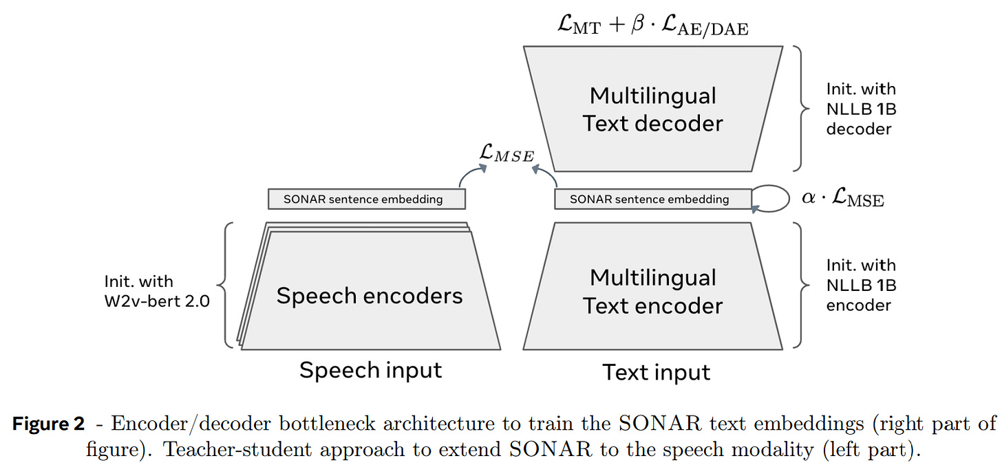
   1. Encoder-decoder architecture for text and speech.

   2. performs character level tokenization of sentence

   3. uses universal encoding space for multi/cross-lingual data (the model is Pre-trained in such a way that sentence from multiple languages pointing to same information/having same meaning share/have similar representations).

   4. for speech-text alignment, teacher student learning is used (teacher could be text model and student could be speech encoder, this is a common alignment practice for distillation), i.e for a given text and it's corresponding speech they have to generate/share similar embeddings.

      

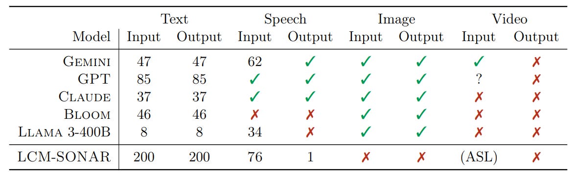
      Comparison of language and modality coverage for several LLMs and our LCM operating on the SONAR embedding space.

Outcome

1. Performs multiple tasks like abstractive summarization, long context reasoning on-par with model from same size category, which showcases that the proposed method works.

   

2. The Diffusion based LCM works better than other two methods, and is a preferred choice for paraphrasing and content generation.

   

3. A different modeling choice opens up doors for more experiments and research, imagine the implication of replacing PreNet and PostNet with a deterministic space (like a Dodecahedron or Torus).
   

   

---

Thoughts

1. The BLT architecture could be used here for encoder and decoder, leading to a more scalable architecture.

2. The model operates on single level of information hierarchy, it's like always thinking in sentences, instead of words, phrases or clauses. A hierarchical LCM could be implemented with some loss aggregation for more robust architecture.

3. Work over Knowledge extension, how can we apply PEFT (Parameter Efficient Fine-tuning) here for extending knowledge at concept level.

4. Testing with fixed manifolds with known boundary conditions to understand the behaviour of knowledge on complex surfaces.

   

   ---

   What we learnt today?
   

1. We discussed how selective bias at certain places could be helpful.

2. The ideology behind LCMs and how it decouples concept and language.

3. We dived deep into architecture choices and modules.

4. We concluded with further advancements and potential research ideas/directions.

   ---

   
   Paper link :
   For further nuances and details, please go through the paper here : https://arxiv.org/pdf/2412.08821

   That's all for today.

   We will be back with more useful articles, till then happy Learning. Bye👋

1. https://arxiv.org/abs/2310.04378